<?xml version="1.0" encoding="utf-8"?><feed xmlns="http://www.w3.org/2005/Atom" ><generator uri="https://jekyllrb.com/" version="3.10.0">Jekyll</generator><link href="https://macklin-cordes.com/feed.xml" rel="self" type="application/atom+xml" /><link href="https://macklin-cordes.com/" rel="alternate" type="text/html" /><updated>2026-04-30T14:13:36+00:00</updated><id>https://macklin-cordes.com/feed.xml</id><title type="html">Dr Jayden Macklin-Cordes</title><subtitle>Computational linguist · Language evolution · Bayesian methods</subtitle><author><name>Jayden Macklin-Cordes</name><email>jayden@macklin-cordes.com</email></author><entry><title type="html">Chromatography</title><link href="https://macklin-cordes.com/posts/2026/04/chromatography/" rel="alternate" type="text/html" title="Chromatography" /><published>2026-04-22T00:00:00+00:00</published><updated>2026-04-22T00:00:00+00:00</updated><id>https://macklin-cordes.com/posts/2026/04/blog-post-5</id><content type="html" xml:base="https://macklin-cordes.com/posts/2026/04/chromatography/"><![CDATA[<p>Just want to know how to actually use the thing? <a href="#actually-using-it">Jump here</a></p>

<h2 id="the-habit">The habit</h2>

<p>I have a <del>quiet</del> colourful habit. Whenever I’m selecting colours for a slide presentation, a poster, or data visualisation for a paper, I start digging through my own photos.</p>

<p>A plum red taken from Uluru at sunset, the blue of the ocean at Bar Beach, a green from the back of a king parrot. This personal touch feels satisfying, even if no one else knows where the colours came from (or, likely, they don’t even have a conscious thought about the colours at all). It’s a fun way to re-engage with something I created in the past (which would otherwise tend to sit underappreciated in my photos app), and remix it into something completely new.</p>

<p>And honestly? I find that the results are typically as good as, or better than, off-the-shelf palettes from the usual online sources. Often, I’ll spend time trawling through sources like <a href="https://colorbrewer2.org/">ColorBrewer</a> (excellent resource, not knocking it), but whatever I pick will feel unsatisfactory in some way, or just too generic. After some time of being overly particular about my colour choices, I’ll find myself going back to my photo collection to find something that really hits the spot. I suppose that a palette which emerges from a real photographic composition will have a particular kind of internal coherence that hand-composed palettes often struggle to replicate. The colours coexisted in a real place, sharing the same light and atmospheric conditions, and they already caught my eye when I framed the shot in the first place.</p>

<p>This process, though, has always been slow, manual and non-replicable. I’ll scan my photos for one that broadly has the kind of palette I’m after. I’ll take in the details of the picture and use macOS’s Digital Color Meter to find the right pixels with the colours I want. Then I’ll take note of the RGB values, one at a time, convert to hex, and paste into my R script, CSS or whatever. I don’t record which photo was used to create the palette, so next time I start a project a few months down the road, I’ll either copy the palette I used last time (losing the personal touch, since I forgot where it came from) or start the whole process anew with a different photograph.</p>

<p>Lately, I’ve been on a mission to codify something of a ‘visual identity’. Partly for (erm, wanky) self-promotional reasons, but also with the practical aim of reducing the amount of time I spend agonising over minor, recurring design decisions when I’m writing talks and making things.</p>

<p>I created this app initially for personal use. I just wanted something to help me craft attractive, personal colour palettes from my own photography, make tricky colour swatch decisions once, and save the output for safe keeping. It turned out kinda cooler than expected though, so now I’m releasing it publicly.</p>

<h2 id="chromatography">Chromatography</h2>

<p><a href="https://chromatography.pages.dev/">Chromatography</a> is a free, browser-based tool for pulling colour palettes out of your own photographs. You drop in an image and tell it how many colours you want. The app extracts a palette automatically, and you can then refine that palette. You can sample additional colours with an eyedropper, drag/reorder swatches, adjust lightness or hue with sliders, and check contrast ratios for accessibility. When you’re happy, you can export the result in a variety of formats: CSS, JSON, R snippet ready for ggplot, GIMP’s GPL, Markdown, or a standalone HTML guide. Everything runs locally in your browser. No images are uploaded to a server. There is no backend, no bloat, no paywall/freemium model, and no account to sign up for.</p>

<p>To reiterate, I started this project for myself. I just wanted to do my thing — extract a palette from my photo of choice, potentially tweak it, and save it for future use — without the friction of my usual manual method. It wasn’t intended to be a public-facing product. Pretty quickly though, it started to feel like something with the potential to be a unique, useful app. The ability to straightforwardly extract a palette from an image in this way, with the combination of perceptually-correct colour handling, sub-pixel manual sampling, modern contrast scoring, gamut feedback, and multi-format export, to the best of my knowledge, isn’t really matched by comparable free tools nor potentially even paid ones. And the whole application fits in a single React component under 100 kB.</p>

<p><img src="/images/chromatography-home.png" alt="Chromatography home page" /></p>

<h2 id="how-it-works">How it works</h2>

<p>If you want to extract a palette from a photograph automatically, the naïve approach is: look at every pixel, cluster the pixels into N groups based on how similar their colours are, and pick a representative colour from each group. This is basically what every palette-extraction tool does. The interesting questions are (a) what do you mean by “similar”?, and (b) how do you cluster?</p>

<p>Consider similarity first. Computers by default represent colour in <em>RGB</em> space, which is how your monitor mixes light to produce the picture you see. RGB is convenient because it maps onto hardware, but it’s a poor representation of human <em>perceptual</em> difference. In RGB space, a colour is represented by a set of three values, specifying how much <em>R</em>ed, <em>G</em>reen, and <em>B</em>lue to mix. Two pairs of RGB triples that are the same Euclidean distance apart can look wildly different to the eye — a shift of twenty units in a dark blue might be barely visible, while the same shift in a bright yellow might look like a completely different colour. If you ask a computer, which only knows colours as a set of RGB numbers, not as we humans really see them, it’ll produce a set of nicely spaced RGB number values, but those won’t actually correspond to anything we’d see as a well-balanced colour palette.</p>

<p>What you want is a colour space in which equal (numeric) distances correspond to equal perceived differences. There’s been decades of work on this in colour science, and arguably the current leader is <a href="https://bottosson.github.io/posts/oklab/"><em>OKLab</em></a>, introduced by Björn Ottosson in 2020. OKLab is designed so that its coordinates align with human perception, while addressing some of the drawbacks of older perceptual spaces (e.g., CIELAB, CIELUV) particularly relating to hue and lightness. Chromatography does all of its clustering and comparison in OKLab. When you see a palette extracted from one of your photos, what you’re seeing is the result of asking: of all the regions of perceptual colour-space this photo occupies, where are its natural centres?</p>

<p>The clustering algorithm is <em>k-means++</em>, a small but important refinement over vanilla k-means. Vanilla k-means picks its starting centroids at random, which can land you in terrible local minima: you extract a palette, two of your six colours turn out to be nearly-identical shades of the same thing, and a whole region of the image goes unrepresented. k-means++ picks its starting centroids probabilistically, with new centroids preferentially chosen to be far from the existing set. Very little extra computational cost, but much better starting conditions.</p>

<p>The manual sampling and editing side adds an extra layer of control over the whole process. This is one point of difference from many of the other palette extraction tools online, which just give you an automatically-extracted set of colours and then you have take it or leave it. I think it’s important to remember that there isn’t a single, deterministic, mathematically optimal solution to picking a set of colours from a photograph. There’s still room for a little art in the science of colour palette extraction. And what looks good in a photograph is sometimes not precisely 1:1 with what works in data visualisation (especially where sequential or diverging palettes are concerned).</p>

<p>The loupe feature displays the colour under your cursor, computed at sub-pixel resolution by interpolating between the surrounding pixels. Click to add the colour to your palette. I deliberately designed it so you can’t click and drag an existing point on the picture. If you have a colour that is nearly but not quite right, the correct approach is to scan around nearby in the image, find something you’re happy with and add it, then delete the previous one from your palette. This prevents shifting an existing colour in the palette then being unable to recover it again if you can’t find something better nearby or change your mind.</p>

<p>Colour swatches can be nudged in <em>OKLCH</em>, the polar form of OKLab (L for lightness, C for chroma, H for hue). Editing in OKLCH rather than HSL means that rotating the hue doesn’t change the perceived lightness, and pulling the chroma doesn’t accidentally shift the hue. If you’ve ever wondered why fiddling with HSL sliders never quite gives you what you want, this is also why. If you end up unhappy with any adjustments, there is a back button which resets the colour to what was originally extracted from the photograph.</p>

<p>Finally, contrast. Maintaining sufficient contrast between text and background colours is important for accessibility, but it’s also just more pleasant even with full vision. Web accessibility conventions for the last decade have used WCAG 2’s contrast ratio, but this doesn’t take into account perception and thus tends to fail in predictable ways. It’s based on a crude luminance division that systematically misestimates perceived contrast for mid-tones and dark-on-dark pairs. The draft replacement, <em>APCA</em> (the Accessible Perceptual Contrast Algorithm, by Andrew Somers), is polarity-aware and better aligns with how human eyes distinguish text from background. Chromatography uses APCA. Every swatch in your palette is scored against cream, white, and black, in both text-on-background and background-on-text directions. Finally, different text types require different levels of contrast — large title text doesn’t require quite as much contrast as small body font, for example. Different minimum thresholds for different text types are suggested at the bottom of the contrast panel. It’s worth keeping an eye on this if any of the colours in your palette are going to be paired with, or used for text.</p>

<h2 id="actually-using-it">Actually using it</h2>

<p>The intended pipeline is pretty straightforward. Start by dropping a photo into the workspace. Select how many colours you’d like Chromatography to extract (six by default, adjustable from two to twelve). If you like what came out, happy days. You might reorder swatches by lightness or hue, hit Export, and go.</p>

<p>Keep in mind that k-means++ is stochastic (there’s an element of randomness every time). I deliberately kept it unseeded, so each time you click Extract, it’ll run fresh and give a different result. Usually it’s pretty stable, so the differences are slight (particularly when extracting a larger number of colours). But it means that if you’re unhappy with the starting point, you can simply click and try again. Often it’s worth rolling the dice a few times until you get a good serviceable starting point.</p>

<p><img src="/images/chromatography-loupe.png" alt="Chromatography loupe" /></p>

<p>If you want to refine, there are two main levers. The eyedropper lets you click anywhere on the image to add a manually-chosen colour to your palette. The per-swatch panel exposes sliders for lightness, chroma, and hue, plus a revert button that resets the swatch to its original sampled value if you OKLCH too close to the sun. You can drag swatches around to reorder; you can sort them by perceptual criteria (lightness, chroma, hue, pixel weight); you can save the whole project to a JSON file that contains both the swatches and the source image, and reload it later to pick up where you left off.</p>

<p>When you’re done, there are several Export options: CSS custom properties for web work, JSON for anything programmatic, an R code snippet for use with ggplot, a GIMP Palette (.gpl) for desktop graphics. There is also a Markdown option for documenting the palette, and standalone HTML for sharing a rendered guide.</p>

<p><img src="/images/chromatography-adjust-panel.png" alt="The colour adjustment panel" /></p>

<h2 id="a-note-for-data-visualisation">A note for data visualisation</h2>

<p>A good chunk of my own use for Chromatography is academic: slides, posters, figures. On the figures side, a caveat is warranted. <em>Palettes from photographs tend to work well only for categorical data.</em> The colours in a photograph aren’t ordered along any single perceptual axis; they’re scattered across the colour space. This maps naturally onto categories, which also have no intrinsic order, but not onto numeric scales, which need monotonic lightness (for sequential scales) or balanced lightness around a midpoint (for diverging ones). With some work, you can coax a sequential scale out of a photograph by picking swatches along one axis and using the sliders to push the extremes brighter or darker, but ymmv. For categorical palettes, though, where the job is to be distinguishable and harmonious rather than to encode magnitude, I find that photographs often work as well as anything online.</p>

<h2 id="the-writeup-companion">The writeup companion</h2>

<p>If you’re planning to reuse a palette over time, it’s useful to have some documentation of it. This is the idea behind the Markdown export option. It should record, at a minimum, a palette title for you to refer back to, a reminder of the image it came from, a list of the colours, and a description of what they’re used for (what’s the primary colour, secondary colours, highlight colour, body text colour, and so on). This doubles as a handy guide if you’re working with AI — just give Claude (or whoever) your palette guide and it can produce output matching your preferences.</p>

<p>The Markdown export function will give you a nice template, with your selected colour specifications pre-filled, and then you can fill in the details yourself. Alternatively, writing this kind of guide is something that large language models are quite well suited for.</p>

<p>I considered implementing some kind of LLM integration for this task. But Chromatology is a lightweight, static web app with no backend. It would have massively complicated things and required a heap of server side computation to implement this. It felt like an overly heavy-handed option, so I let it stand in its current, nice, client-only shape.</p>

<p>As a compromise, I’ve published a companion ‘prompt pack’ on GitHub. This is a carefully designed system prompt and template that you can paste into Claude (or your LLM of choice) along with your palette’s JSON export. I’ve tried to steer it away from generic sensory prose (“a rich, moody blue evokes the ocean’s depths”) or overly dramatic colour names (“Whispering Midnight Wanderlust”). The prompt asks for more restrained, descriptive language:</p>

<div class="language-plaintext highlighter-rouge"><div class="highlight"><pre class="highlight"><code>Two or three words maximum. They should be evocative but restrained — 
the kind of name a paint manufacturer with taste would use, not the 
kind a scented-candle company would. "Winter slate", "wet sandstone" 
— good. "Ethereal Oceanic Dreams" — no.
</code></pre></div></div>

<p>The full prompt <a href="https://raw.githubusercontent.com/JaydenM-C/chromatography/refs/heads/main/writeup_prompt_README.md">lives in the GitHub repo</a>. Export your palette as JSON, paste both into a fresh Claude conversation, et voilà.</p>

<p>I also recommend asking for an HTML rendering and/or mock-up, especially if you have some nice font/typeface choices ready to go as well. I find Claude does quite a good job at this.</p>

<p>(It might also be fun to play around with prompt variations. What happens if you ask for overly poetic, dramatic descriptions?)</p>

<h2 id="two-worked-examples">Two worked examples</h2>

<p>I’m still in the very early days of experimenting with this app myself. But uh, here’s a little something I prepared earlier…</p>

<p><img src="/images/chromatography-maritime-source.jpeg" alt="Fishermen on sandstone cliffs over ocean" /></p>

<p>The first example is a sandstone+sea palette. I took it from the ANZAC Memorial Bridge in Newcastle. The golden afternoon sun on sandstone provides a really nice contrast to the blue ocean, and I enjoyed the bright red jacket highlight. Here’s the palette applied as a design mock-up:</p>

<iframe src="/files/chromatography/maritime-mockup.html" style="width:100%; height:820px; border:none;" loading="lazy"></iframe>

<p>This is a fairly cool-toned palette, and I’m more of a warm palette guy, so I probably wouldn’t use this myself. But still, neat.</p>

<p>The second example is a palette called “Fired Clay” (warm ochres, a muted aubergine, a pair of pale sandstone tones) with a full guide generated by the writeup prompt I mentioned earlier:</p>

<iframe src="/files/chromatography/palette-guide.html" style="width:100%; height:820px; border:none;" loading="lazy"></iframe>

<p>Which picture generated this warm, earthy palette, you ask? I’ll let you imagine some possibilities for a bit. When you’re ready, scroll to the bottom of this article.</p>

<p>I’m not sure what this says about the relationship between aesthetic judgement and the underlying thing being judged…</p>

<h2 id="keeping-things-light">Keeping things light</h2>

<p>This is a simple app with a specific, fairly niche use case. Still, I’m quietly pleased with just how lightweight it is, and how easy it’s been to deploy. As I mentioned, the entire thing is a React web app under 100kB. No backend, no database, no telemetry other than a simple view counter. There are no external dependencies except Google Fonts. No picture you upload gets touched by an outside server, much less saved anywhere outside your own machine. Nevertheless, there’s a nifty amount of functionality which in some respects even exceeds Adobe’s online colour palette extractor. All without being hassled by popups or login prompts.</p>

<p>I wouldn’t want to make too much of a broad, proselytising claim about software development on the basis of a simple colour picker. But there’s probably a lesson in here on the value of well-chosen primitives. I was able to keep things lean by standing on the shoulders of others — OKLab, k-means++ and APCA. There’s a world in which I started with classic defaults (RGB, vanilla k-means, WCAG 2), then spent enormous effort patching around RGB’s poor perceptual behaviour, adding re-roll buttons to rescue users from k-means’ local minima, and working around WCAG 2’s misleading mid-tone contrast readings. The result would’ve been considerably more surface-level complexity, and a more bloated app.</p>

<h2 id="where-to-next">Where to next</h2>

<p>I’ve momentarily paused development of Chromatography to give the current (beta-ish) iteration a proper test run. Several candidate v2 features are on my mind though. One option that stands out is <em>region-based sampling</em>: drawing a box or polygon around part of an image and extracting a palette from that region specifically, rather than the whole frame. This would make it possible to, say, extract a palette specifically from a bird or a flower, without including the background. This would further distinguish the app from other palette-from-photo tools online.</p>

<p>A mobile-friendly UI is another possibility. I anticipate Chromatography will be most useful on desktop anyway, but currently it breaks completely on mobile, which feels sad.</p>

<p>There are other candidates: chroma-preserving gamut mapping, data-visualisation-specific palette generation modes, seeded extraction for reproducibility, persistence via IndexedDB. But I’ll wait a bit and see where the main friction points are. Feel free to make feature requests via <a href="https://github.com/JaydenM-C/chromatography/issues">GitHub issues</a>.</p>

<h2 id="links">Links</h2>

<p>Chromatography is free and lives at <a href="https://chromatography.pages.dev/">chromatography.pages.dev</a>.</p>

<p>The code is open source (GPL v3) on <a href="https://github.com/JaydenM-C/chromatography">GitHub</a>; bug reports and pull requests welcome.</p>

<p>If you find it useful and feel like chipping in a few quid toward ongoing development, my <a href="https://ko-fi.com/jaydenmacklincordes">Ko-fi page</a> is here.</p>

<p>If you extract a palette you’re fond of, I’d love to see it. Send a screenshot or a link through any of the usual places. Maybe I can create a central repository of palettes, if anyone feels inclined to share their work!</p>

<p><img src="/images/chromatography-fired-clay.png" alt="&quot;Fired clay&quot; palette source" />
<em>“Fired clay”</em> indeed.</p>]]></content><author><name>Jayden Macklin-Cordes</name><email>jayden@macklin-cordes.com</email></author><category term="data visualisation" /><category term="design" /><category term="tools" /><category term="photography" /><summary type="html"><![CDATA[I have a colourful habit.]]></summary></entry><entry><title type="html">Phonotactics in historical linguistics (Part II)</title><link href="https://macklin-cordes.com/posts/2026/03/phonotactics-in-historical-linguistics-2/" rel="alternate" type="text/html" title="Phonotactics in historical linguistics (Part II)" /><published>2026-03-23T00:00:00+00:00</published><updated>2026-03-23T00:00:00+00:00</updated><id>https://macklin-cordes.com/posts/2026/03/blog-post-4</id><content type="html" xml:base="https://macklin-cordes.com/posts/2026/03/phonotactics-in-historical-linguistics-2/"><![CDATA[<p>A few years ago, I did the thing where you write the thing, and now I’m legally entitled to sow confusion by shouting “I’m a doctor!” during medical emergencies on planes<sup id="fnref:1" role="doc-noteref"><a href="#fn:1" class="footnote" rel="footnote">1</a></sup>. In a previous post <a href="https://macklin-cordes.com/posts/2022/01/phonotactics-in-historical-linguistics/">(Part I)</a>, I wrote about the background and motivation behind the PhD project that kept me busy for so long. But I left it on a cliffhanger. The big question driving my PhD was whether I could build better family trees of languages (<em>phylogenies</em>) by combining traditional cognate data (sets of related words across languages) with a new kind of data extracted from <em>phonotactics</em>, the rules governing which sounds are allowed to appear together. At the end of the post, I promised a Part II discussing what I actually found. Four short years later, here it is. I appreciate your patience.</p>

<p>To briefly recap: the appeal of phonotactic data is twofold. First, a language’s phonotactic restrictions tend to be historically conservative — even when languages borrow vocabulary from their neighbours, they tend to reshape those borrowed words to fit their own sound rules (I’m sure you all remember the <em>kurisumasu</em> and <em>meli kalikimaka</em> examples from Part I like it was yesterday 😉). Second, you can extract a lot of phonotactic information straight from a wordlist using automated methods, which is a huge advantage for understudied language families where detailed cognate data doesn’t yet exist.</p>

<p>Before I could answer the main question, though, I had to do some groundwork. I needed to understand the data itself — what does it look like, statistically? Then I needed to check whether phonotactic data actually carries any historical information at all, before attempting to feed it into a tree-building algorithm. Only then could I run the big experiment. What follows is the story of that process. And, fair warning, the ending isn’t quite the fairytale I expected.</p>

<h1 id="what-does-the-data-actually-look-like">What does the data actually look like?</h1>

<p>Before you pour data into a fancy algorithm, you should probably understand the data itself. What shape does it have? What patterns does it follow? What does that tell you about the forces that produced it? This is the eat-your-vegetables portion of the thesis — not the flashiest part, but it earns its place later.</p>

<p>Here’s the question. Every language has a set of contrastive speech sounds — its <em>phonemes</em>. Some of those phonemes are very common in the language’s vocabulary and others are quite rare. If you rank a language’s phonemes from the most frequent to the least, what pattern do you get? Is it a gentle slope, with most sounds appearing at roughly similar rates? Or is it something more dramatic?</p>

<p>It turns out to be dramatic. The pattern you see, again and again across different languages, is a sharply skewed curve: a handful of phonemes are extremely common, and then there’s a long tail of many phonemes that are relatively rare. If you rank UK cities by population, you get a similar kind of shape (Figure 1). London towers over everything, Birmingham and Manchester are a distant second and third, and then there’s a long, flat tail of dozens of cities from Leicester down to Guildford that are all roughly the same size relative to London. This kind of heavily skewed distribution pops up all over the place in nature and human society, from the popularity of websites to the distribution of earthquake magnitudes. In linguistics, it’s associated with George Zipf, who observed that word frequencies in a text follow a similar pattern (the most common word appears roughly twice as often as the second most common, three times as often as the third, and so on) — hence you may hear references to “Zipfian” distributions, or “Zipf’s Law”.</p>

<figure style="display: flex; flex-wrap: wrap; gap: 12px; justify-content: center;">
  <img src="https://macklin-cordes.com/images/walmajarri-phonemes.png" alt="Bar chart of phoneme frequencies in Walmajarri. The chart is quite skewed, such that the few most frequent phonemes are much more frequent than the rest." style="flex: 1 1 300px; max-width: 75%; height: auto;" />
  <img src="https://macklin-cordes.com/images/uk_cities_rank_size.png" alt="Chart of UK city populations. The plot is even more skewed than Walmajarri phonemes. London is massively larger than the next largest, Birmingham and Manchester, followed by a long, flat tail of 47 much smaller cities." style="flex: 1 1 300px; max-width: 75%; height: auto;" />
  <figcaption style="flex-basis: 100%;">Left (or top): Phoneme frequencies in Walmajarri, an Australian Indigenous language. Right (or bottom): UK cities ranked by population. Heavily skewed patterns recur again and again throughout the 166 languages in my sample, and indeed throughout nature and society generally. But do phoneme frequencies truly follow Zipf's Law? It turns out it's a bit more complicated.</figcaption>
</figure>

<p>Previous researchers had claimed that phoneme frequencies follow this same Zipfian pattern. But there was a problem: the statistical methods they’d used to evaluate this had since been shown to be unreliable. So, using more robust methods and a dataset of 166 Australian languages, I re-evaluated the question. What I found was more nuanced than the earlier picture. The most frequent phonemes in a language do follow something like a Zipfian, power law pattern — a “rich-get-richer” dynamic where the already-common sounds tend to attract even more usage. But the least frequent phonemes follow a different pattern entirely, one better described by an exponential distribution, which is associated with simpler “birth-death” processes where sounds come and go at some characteristic rate. In other words, a kind of split personality: one pattern governing the top of the frequency ranking and a different pattern governing the bottom.</p>

<p>Why should we care about any of this? Two reasons. First, different mathematical distributions point to different underlying causal processes. If we can identify the right distribution, we’re getting a clue about the forces — sound changes, borrowings, mergers, splits — that shape a language’s phoneme inventory over time. That’s intrinsically interesting, but it also matters practically, because if you want to build an evolutionary model of how these frequencies change along a family tree, you need to know what you’re modelling. Second, this result was an early warning sign. The data has a complex, composite structure — it doesn’t follow one neat pattern — and that means capturing it faithfully in a statistical model is going to be difficult. A point I would come to appreciate more fully later on.</p>

<h1 id="is-there-a-trace-of-history-in-phonotactics">Is there a trace of history in phonotactics?</h1>

<p>The previous section looked at the frequencies of individual sounds. A useful starting point, but not quite where the action is. Remember, it’s <em>phonotactics</em> that I hypothesised to be historically conservative — the rules governing which sounds are allowed to appear together, not just how often individual sounds crop up. So the natural next step was to turn to the frequencies of sequences of sounds, pairs of adjacent segments called <em>biphones</em>. This also has the happy side effect of giving far more data to work with per language (a language might have only 20-odd phonemes, but hundreds of biphone sequences). It’s all very well that phoneme frequencies have interesting statistical properties. But the real question for my project is whether phonotactic data, the rules and frequencies governing how those phonemes fit together, actually contain historical information. Do closely related languages resemble each other phonotactically more than distant ones? If not, the data is just noise as far as phylogenetics is concerned, and I can pack up and go home.</p>

<p>The concept I needed is called <em>phylogenetic signal</em>. The idea is simple enough: if some trait has evolved along a family tree, then closely related species (or languages) should resemble each other more than distantly related ones, and more than you’d expect by chance. Think of it like family resemblances. Siblings tend to look more alike than cousins, who tend to look more alike than strangers<sup id="fnref:2" role="doc-noteref"><a href="#fn:2" class="footnote" rel="footnote">2</a></sup>. That’s a consequence of shared ancestry — more specifically, the <em>relative amount</em> of shared ancestry (siblings have shared ancestry down to the parent generation, cousins have shared ancestry down to the grandparent generation). The same logic applies to languages. If phonotactics evolves along a language family tree, then closely related languages should have more similar phonotactic patterns than distant relatives. And crucially, there are statistical tests that let you quantify this — to measure not just whether the resemblance is there but how strong it is.</p>

<p>So I took phonotactic data from 112 languages from the Pama-Nyungan family, a large family of Indigenous Australian languages spanning about 90% of the continent. I then compared the data against a known family tree that had been built independently from cognate data (the traditional, gold-standard way to build language trees). The test: does the phonotactic variation across these languages line up with what we’d expect if it had evolved along that tree? I ran this test on three progressively finer-grained datasets. The first was binary — for each pair of adjacent sounds (a biphone), does it occur in a language’s vocabulary or not? This is the coarsest level of information: a simple yes or no. The second recorded the actual frequencies of transitions between individual sounds — not just whether a sequence occurs, but how often. The third grouped sounds into natural classes (categories like “nasal” or “velar” that reflect how and where in the mouth a sound is produced) and recorded transition frequencies between those classes.</p>

<figure>
  <img src="https://macklin-cordes.com/images/PN_tree_pruned.png" alt="A phylogenetic tree of 112 Pama-Nyungan languages, showing branching relationships inferred from lexical cognate data. The tree fans out from a single root on the left into many branches on the right, with language names at the tips." style="max-width: 100%; height: auto;" />
  <figcaption>The Pama-Nyungan reference tree, inferred from lexical cognate data by Claire Bowern. The numbers indicate confidence in each branching point: above 0.8 is pretty confident, below 0.5 is 🤷‍♂️. This tree is the yardstick I tested my phonotactic data against. The question: does phonotactic variation across these 112 languages line up with the branching structure in this tree?</figcaption>
</figure>

<p>The result was clear, and if it wasn’t yet time to pop some champagne corks, it was at least time to grab a couple of bottles and put them on ice. All three datasets showed statistically significant phylogenetic signal. But the strength of that signal increased markedly as the data got more fine-grained. The binary data — the simple yes-or-no — showed the weakest signal. The frequency data was stronger. And the natural-class-based frequency data was strongest of all. This makes intuitive sense: there’s far more information in how often a sound sequence occurs than in merely whether it occurs. And grouping sounds into natural classes captures something real about how sound change actually works — sound changes tend to affect whole classes of sounds (all the nasals, say), not just individual phonemes one at a time.</p>

<p>What made this result especially striking is that Australian languages have long been described as phonotactically uniform. The conventional wisdom was that there just wasn’t much phonotactic variation to find. And at a coarse, binary level, that’s partly true — many of the same sound sequences are permitted across most Australian languages. But once you look at the frequencies, a different picture emerges. There’s a rich layer of variation hiding beneath the surface, and that variation patterns phylogenetically. The historical signal was there all along; you just needed the right resolution to see it.</p>

<p>So, phonotactics carries genuine historical information. In principle, this data could help build better family trees of languages. I could stop here, on this high note, and give the impression that phonotactics is the answer to all our phylogenetic prayers. But that would be only half the story. Don’t pop those champagne corks just yet…</p>

<h1 id="the-big-experiment">The big experiment</h1>

<p>Time for the real test. But detecting a signal and using it to infer a tree are very different propositions. To actually put this to the test, I needed to combine phonotactic data with traditional cognate data, feed both into the Bayesian tree-building machinery, and see whether the result was any better than what you’d get from cognates alone.</p>

<p>Back in Part I, I gave some background on Bayesian computational approaches to phylogenetic tree inference. And, in particular, I described a process called MCMC (Markov Chain Monte Carlo), where the computer generates millions upon millions of random trees and gradually homes in on the best solutions. This is the approach I took here. It’s finally time to see it in action. I set up two competing models for a sample of 44 western Pama-Nyungan languages. In the first model, the computer builds a single tree from both the cognate data and the phonotactic data together. In the second, it builds two separate trees — one from cognates, one from phonotactics — independently of each other. If the phonotactic data genuinely helps, then the combined model should fit the data better than keeping the two data sources apart. The method for comparing models is technical, but the underlying question is simple: does adding phonotactic data make the tree better, or not?</p>

<p>It did not.</p>

<p>Or, more precisely: the experiment failed to produce a clear answer, which is arguably worse than a clean negative result. The models with phonotactic frequency data never properly stabilised. Remember those MCMC trace plots from Part I — the ones that show the computer’s likelihood score at each iteration, and how they’re supposed to settle into a nice, stable plateau? Mine looked like abstract art. Some chains would wander around aimlessly for tens of millions of iterations. Others would appear to converge, then abruptly lurch somewhere else. No amount of praying to the Bayesian gods would suffice to make them behave. The upshot is that the statistical comparison between models was unreliable. I couldn’t trust the numbers.</p>

<figure>
  <img src="https://macklin-cordes.com/images/sep_trace_dens_ch1-10.png" alt="MCMC trace plot showing ten chains that fail to converge, instead settling into distinct bands at different likelihood levels across 100 million iterations." style="max-width: 100%; height: auto;" />
  <figcaption>What MCMC convergence failure looks like. Each coloured line is an independent chain — they're supposed to settle into the same band (compare with the well-behaved trace in Part I). These ones did not get the memo.</figcaption>
</figure>

<p>What I could glean from the wreckage was not encouraging. The best average tree produced by the combined model came out oddly flat — a squished, star-like structure with weaker branching than you’d get from cognates alone. In tree-building, a flat tree is a tree that’s not really saying much. It’s the phylogenetic equivalent of a shrug. This suggested that the phonotactic data, rather than adding useful historical signal, was introducing a bunch of noise that washed out the branching structure.</p>

<p>Why did it go wrong? The core problem was a tension between making the evolutionary model realistic and making it computationally feasible. The model I used assumed that phonotactic frequencies change gradually over time — drifting up and down at random, a process called Brownian motion. This is a reasonable starting point and it’s a standard model available in existing phylogenetic software. But real sound change doesn’t work like that. When a language undergoes, say, a phonemic merger (two formerly distinct sounds collapse into one<sup id="fnref:3" role="doc-noteref"><a href="#fn:3" class="footnote" rel="footnote">3</a></sup>), the frequencies of affected sound sequences don’t drift gently downward. They jump, suddenly, to zero or one. And when new sound distinctions emerge, the reverse happens: frequencies leap from zero to some non-trivial value overnight. A model that only allows for gradual drift is going to struggle with data that’s shaped by sudden jumps. On top of this, I had to treat every phonotactic variable as if it were evolving independently of every other — which is linguistically absurd, since sound changes affect whole classes of sounds at once. But modelling the dependencies between thousands of variables would have been computationally intractable. So I made the simplification, knowing it was wrong, because the alternative was not running the experiment at all.</p>

<p>This is not the fairytale ending you want for the final chapter of your PhD. Put that champagne back in the fridge.</p>

<h1 id="what-i-learned">What I learned</h1>

<p>A PhD that ends with “it didn’t work” sounds dispiriting (and trust me, I’ve spent plenty of time feeling dispirited about it). But, especially with some time and distance to reflect, I realise that isn’t quite right. The result was indeterminate, not negative. The experiment didn’t show that phonotactics is useless for phylogenetics — it showed that the tools I had weren’t yet adequate for the job. Those are very different conclusions, even if they felt similar at 2am during the depths of late-stage thesis-writing hell.</p>

<blockquote>
  <p>“If you’ve made up your mind to test a theory, you should always decide to publish it whichever way it comes out. If we only publish results of a certain kind, we can make the argument look good. We must publish both kinds of results.” — Richard Feynman</p>
</blockquote>

<p>I take this seriously. If I’d stopped after the phylogenetic signal paper — the beautiful positive result — and never attempted the tree inference experiment, I’d have left a misleading impression that phonotactics was ready for phylogenetic prime time. It isn’t. Not yet. And the field is better served by knowing that than by not knowing it. So did I really spend nearly 5 years of my life investigating a kinda out-there question, which no one was asking, only to find, uh, nothing? I don’t think it’s quite that bleak!</p>

<p>The thesis offers three main contributions. First, it demonstrated that phonotactic data carries genuine historical signal — that the patterns in which sounds are allowed to fit together reflect the evolutionary history of a language family, even in a part of the world where phonotactics was assumed to be boringly uniform. That result stands. Second, it showed that fine-grained frequency data is far richer than coarse binary data for this purpose. If you just ask “does this sound sequence occur: yes or no?” you get a faint signal. If you ask “how often?” you get a much stronger one. Third — and this is the contribution I’m most invested in — it laid out a principled, step-by-step methodology for evaluating any new kind of data in phylogenetics. Rather than just slurping up whatever data we can get our hands on and pouring it into a computational black box, the thesis argues for a deliberate progression: understand the data’s statistical structure, test for phylogenetic signal, evaluate the evolutionary dynamics, and only then attempt tree inference. That framework is generalisable beyond phonotactics.</p>

<p>As for the tree inference question itself, it remains open. To revisit it properly, future work would need better evolutionary models — ones that account for the sudden jumps of sound change rather than assuming everything drifts gradually. It would need smarter ways of handling the dependencies between phonotactic variables, perhaps through phylogenetic factor analysis or linguistically motivated data partitioning. And it would benefit from advances in computational power that are already underway. The problem is hard, but it doesn’t look intractable.</p>

<p>Phylogenetic methods in linguistics are still maturing, and that means you often find yourself innovating, customising or building tools from scratch on the way to answering the question. This can be challenging, but it’s also where the most rewarding work tends to happen. There’s a wide gap between “this data contains useful information” and “we can successfully use this data in a model,” and bridging it requires the kind of slow, methodical groundwork that doesn’t make for a flashy conference talk — but without which the flashy results would be built on sand. For the sake of the world’s under-resourced languages, and the histories they encode, that bridging work is worth doing. And it’s far from finished.</p>

<div class="footnotes" role="doc-endnotes">
  <ol>
    <li id="fn:1" role="doc-endnote">
      <p>Of course I would never do this. But I have watched my share of YouTube videos on how to land a plane, just in case the need should ever arise. <a href="#fnref:1" class="reversefootnote" role="doc-backlink">&#8617;</a></p>
    </li>
    <li id="fn:2" role="doc-endnote">
      <p>To emphasise, this is a <em>general tendency</em>, not an absolute. Sometimes siblings look surprisingly dissimilar, sometimes we find uncanny doppelgangers. But, <em>on average</em>, we expect pairs of siblings to look more similar to each other than pairs of people selected from the population at random. <a href="#fnref:2" class="reversefootnote" role="doc-backlink">&#8617;</a></p>
    </li>
    <li id="fn:3" role="doc-endnote">
      <p>An example is “wh” in English. “Wh” used to be a distinctive sound in English, a voiceless [w̥] (think something like a breathy “hw”). In most varieties of English today, it’s completely collapsed into a single, regular “w” sound. Only a few varieties of Irish, Scottish, and Southern US English still preserve a wh/w distinction. And <a href="https://www.youtube.com/watch?v=7ZmqJQ-nc_s">Stewie Griffin</a>. <a href="#fnref:3" class="reversefootnote" role="doc-backlink">&#8617;</a></p>
    </li>
  </ol>
</div>]]></content><author><name>Jayden Macklin-Cordes</name><email>jayden@macklin-cordes.com</email></author><category term="PhD life" /><category term="linguistic phylogenetics" /><category term="Australian languages" /><summary type="html"><![CDATA[A few years ago, I did the thing where you write the thing, and now I'm legally entitled to sow confusion by shouting "I'm a doctor!" during medical emergencies on planes.]]></summary></entry><entry><title type="html">Rookies into rolled gold</title><link href="https://macklin-cordes.com/posts/2026/03/SC-alchemist/" rel="alternate" type="text/html" title="Rookies into rolled gold" /><published>2026-03-12T00:00:00+00:00</published><updated>2026-03-12T00:00:00+00:00</updated><id>https://macklin-cordes.com/posts/2026/03/blog-post-3</id><content type="html" xml:base="https://macklin-cordes.com/posts/2026/03/SC-alchemist/"><![CDATA[<p>I actually love the footy. It’s weird to say, as a white Aussie dude, but that hasn’t always been the easiest thing to admit. I’ve spent a lot of time floating around the kinds of academic circles where you’re more likely to hear derisive references to “sportsball”. And look, I get it, there’s aspects of footy culture that aren’t always the most attractive. But sport generally has a lot going for it - it’s shaped my whole life. And Australian Rules football, I firmly believe, is one of the most majestic sports of all. It has this kind of beautifully holistic brutality about it. Other sports have individual aspects where they excel - bigger hits, more pure strength, or endurance. But I can think of few if any other sports that demand so much all-round, mentally and physically, of its combatants. The physicality, gut-busting running on a uniquely enormous field, all while executing extraordinarily difficult fine skills, it’s got it all. It’s even uniquely difficult to officiate, requiring an entire third team of elite athletes just to administer the game. I briefly flirted with AFL selection as a boundary umpire, running around in the (now defunct) NEAFL in the early 2010s. I’d regularly run over 20km in a game, and then spend the rest of the day lying in my dark bedroom with a migraine, and then I’d do it all over again the next weekend, because running around the SCG or Manuka Oval and just being a part of the whole thing was <em>really fucking fun</em>. A boundary umpire’s job is largely to run up and down and throw the ball back in play when it goes out of bounds. Even then, just doing a boundary throw-in at NEAFL (RIP) or AFL standard is a specialist skill, requiring specialist training, from a specialist boundary umpire coach, just to be able to do it. The whole thing is bizarre really, and I love it.</p>

<p>Anyway, I’m not here to get in an argument about whether Aussie rules footy is truly the greatest sport on earth. This is all simply to say that I just <em>like</em> it. I like watching it. And I even like supporting the Adelaide Crows, despite the distinct lack of premierships in the last three decades and the damage they inflict on my cardio health every time they play Collingwood.</p>

<p>In my early teens, I had a couple of mates who absolutely lived and breathed sport. We starting playing fantasy football (AFL Supercoach, to be precise) - an online game where you’re given a budget (salary cap), you select a squad of players within the salary cap, and score points based on those players’ real-life performance in AFL matches. We’ve been playing basically ever since. One of these mates has been heroically administering the competition for a number of years now. It’s blossomed into the “Supercoach Legends”, a group of about 30 of us, competing in a three-tiered league complete with promotion and relegation, cash prizes, and a breathtaking flood of banter every March through to September.</p>

<p>For a number of years now, it’s occurred to me that selecting an AFL Supercoach squad is a problem begging for some computational optimisation. At the end of the day, it boils down to a pretty simple proposition: Maximise points per dollar spent. Each year, I think about how cool it would be to make my team selections more data-driven, then I do nothing, then I select my team at the last minute, based largely on vibes. In my defence, until recently, programming a Supercoach team optimiser would have taken far more time and effort than I could afford to spend on a project that isn’t, y’know, work. I made one brief attempt, but my wild idea was to essentially simulate an entire AFL season in R, round-by-round, and it didn’t get very far. A couple of years ago, I thought I’d dabble with this new-fangled thing called ChatGPT to see if that could help. It came up with some reasonable selections …for a team two years prior, when its online training data cut off.</p>

<p>Things are different now. Today’s AI models can find and distill all the latest player news, reason through problems, and write complex code like it’s nobody’s business. So, for Season 2026, I thought I’d treat myself to some Claude Opus compute, and have a crack at making the kind of Supercoach optimiser that, until recently, I could have only dreamed of.</p>

<p>Introducing <a href="https://github.com/JaydenM-C/sc-alchemist"><em>SC Alchemist</em></a>.</p>

<hr />

<h2 id="what-is-afl-supercoach">What is AFL Supercoach?</h2>

<p>If you’ve never played AFL Supercoach, the gist is thus: you select a squad of 31 AFL players, staying within a fixed salary cap, and each week your on-field team earns points based on how those real-life players actually perform. Disposals, marks, tackles, hitouts, clearances — every statistical action on the field translates to a Supercoach score. A gun midfielder having a dominant game might score 140 points. Some spud who barely got a touch and gave away three free kicks? Maybe 20.</p>

<p>The game runs throughout the AFL season, rounds 1 through 24 (not finals). Each week you’re competing head-to-head against others in your league (my fellow Supercoach Legends), and against all 200,000+ other coaches in an overall rankings table. You have a limited number of trades to move players in and out over the course of the season. The aim isn’t just to pick a good team on day one; it’s to manage and evolve your squad across six months of football, navigating injuries, form slumps, unexpected breakouts, and the shifting value of players as their prices rise and fall.</p>

<p>That price mechanism is where things get interesting. Players start the season at a price derived from their scoring history, and that price changes week to week based on their recent scores. A cheap rookie (first-year player) who starts averaging 60+ points per game will rapidly increase in value — and selling them at their peak to fund a top-tier premium is how you build a competitive team. Getting that cycle right, or wrong, can make or break your season.</p>

<hr />

<h2 id="conceptualising-the-problem">Conceptualising the problem</h2>

<p>As you might imagine, the internet is awash with advice on team selection. There is no shortage of journalists, bloggers, podcasters and internet randos on Reddit and Facebook, hyping their predicted breakout stars, arguing about ruck strategy, and discussing the preseason form of the latest crop of rookies. It’s noisy and it’s fun, and there are so many resources these days that it’s hard even for the most time-pressed casual coach to pick a really terrible team. But it also doesn’t exactly produce an optimal team. There’s a lot of groupthink - everyone ends up with the same hyped rookies. There are cognitive biases - everyone overspends on the same ‘safe’ premiums because they fear missing out. And every year, people fall for the same traps - the overhyped mid-pricer who ends up averaging a mediocre 80, or the fallen star who’s surely meant to come good again but, well, stays fallen.</p>

<p>Supercoach is an optimisation problem that most players are solving only approximately, and with a lot of noise. The more you think about it though, the more it becomes apparent that it’s not just a simple matter of dollars in, points out. It’s actually quite a complex, layered optimisation problem.</p>

<p>A key insight is that Supercoach is really a two-phase problem. This will be no surprise to experienced Supercoach coaches, but it’s crucial for the design of any computational optimiser. In the early rounds, the goal isn’t purely point-scoring, it’s <em>generating capital</em>. A cheap rookie who scores 70 per game and rises $150,000 in value over eight weeks is more valuable than a mid-pricer averaging 85, because the rookie funds the upgrade path to a premium averaging 120. In the later rounds, once you’ve converted your cash cows into elite premiums, the game becomes about maximising weekly scores for the run home.</p>

<p>There’s also the concept of positional scarcity. The midfield has fifteen viable premiums in any given year; ruck has maybe three to five. Overspending on the “best” midfielder has lower marginal value than nailing ruck, because the marginal quality difference between mid-tier and top-tier premiums is small in the deeper positions, while in ruck, picking the wrong bloke can structurally hobble your whole season.</p>

<p>Then there’s ownership percentage. If every coach in your league owns Bontempelli, his scores are effectively neutralised. Your edge, playing for your league, comes from correctly-picked unique players, or PODs as they’re known (“players of difference”). High-floor premiums are table stakes; high-ceiling contrarian picks are where you gain ground. This doesn’t intuitively feel like it should matter for the purposes of optimising your team but it can shift risk-reward calculations.</p>

<hr />

<h2 id="building-sc-alchemist">Building SC Alchemist</h2>

<p>The core idea was to build an integer programming optimiser — a branch-and-bound solver that would evaluate every possible combination of players, subject to salary cap and positional constraints, and return the mathematically optimal squad. Unlike heuristics or gut feel, integer programming guarantees the global optimum given the inputs. The challenge, of course, is that the quality of the output is entirely determined by the quality of the inputs. And getting good inputs turned out to be the real work.</p>

<p><strong>Getting the data</strong></p>

<p>The first step was acquiring the player dataset. The AFL Supercoach website is a largely javascript-based application, so there’s nothing to scrape from the HTML directly. Helpfully though, the backend includes a sizeable JSON file containing every player’s price, projected scores, ownership percentage, 2025 averages, and more. It makes an API call to this file whenever you click on a player on the website. This gave me a rich foundation to build on.</p>

<p><strong>The projection problem</strong></p>

<p>The Supercoach website provides its own projected scores, but these were kinda flawed for our purposes (again, no surprise to experienced coaches out there). The projections are heavily weighted toward a player’s record against their specific upcoming opponents. A player facing three difficult early-season matchups might be projected at 75, even if their season-long average is 120. Conversely, a player drawing three weak opponents in the opening rounds gets an inflated projection that the optimiser initially treated as gospel.</p>

<p>The fix was building a blended projection algorithm. For established players with significant game histories, I combined three signals: the 2025 season average (weighted more heavily for players who played more games, using a games-played cap to prevent a 22-game player from completely overriding a 10-game player), the five-round rolling average at the end of 2025 (capturing recent form and trajectory), and the Supercoach website’s three-round projection (capturing fixture difficulty). The result was a projection that was substantially more realistic for long-term season planning.</p>

<p><strong>The rookie problem</strong></p>

<p>Rookies presented a separate challenge. Supercoach’s default projections for inexperienced players are essentially placeholder values based on price tier — they tell you almost nothing about actual likely scoring. Yet picking the right rookies is arguably the single highest-leverage decision in the game. A $100,000 player who averages 80 per game and rises $200,000 in value is transformational. One who gets dropped after two games scores nothing and generates nothing.</p>

<p>This unavoidably requires qualitative research. Thankfully, here again, Claude is useful in a way that is leaps and bounds ahead of even a year or two ago. I set him on the task of scraping community series scores, searching for confirmed role news, identifying players with verified Round 1 starts, and applying domain knowledge about which positions and roles tend to produce reliable rookie scoring. I followed up with some of my own research, and some footy sense as a human who’s watched the game a long time. We went back and forth a bit and together came up with a table of custom rookie projections. They’re not purely algorithmic projections, clearly there’s a degree of distilled vibes baked in, but it still feels considerably more objective than simply making my own educated guesses, or blindly taking some blogger’s own vibes-based projections. And it was certainly a time-efficient process, compared to personally sitting down and watching every preseason match and tracking every draftee over the summer.</p>

<p>I followed up with a very similar hybrid objective-qualitative, iterative, human-AI type process for mid-pricers. To explain: Traditionally, most coaches go for a “guns ‘n’ rookies” strategy, selecting top-tier premium guys, bargain basement rookies for capital growth, and just a small sprinkle of mid-priced guys. Mid-pricers are tricky, because you really need to select them on the basis that you expect them to turn into a breakout premium who you can keep all year. A mid-pricer who scores only mid scores is stuck in a bit of a no man’s land, where they don’t score enough to contribute to your team all season long, but they also don’t generate enough cash to sell or upgrade to someone else, so you’d be better off selecting a cheap rookie who can make good money, and put the savings somewhere else in your team. Consequently, taking a punt on mid-price selections can really make or break your whole team. And predicting which mid-pricers will break out and become premiums in the season ahead is always the most fraught, noisy and hype-filled area of online discussion.</p>

<p>Historically, there are a number of well-known signatures of players with breakout potential: A role-change (e.g. a guy moves into a new, Supercoach-friendly position in his team’s midfield); first year after being traded to a new club (fresh environment, maybe a fresh team role); 22-24 year old players entering their 4th-6th AFL season (entering the prime of their career); players with proven scoring potential who had one bad year (and are therefore discounted in price) due to an injury; and so on. I gave Claude a list of these breakout criteria to look for, and also got him to do a deep dive on mid-priced players who had been the subject of preseason hype. Sometimes the hype is real, so I don’t want to miss out on anyone. But I did give careful instructions to down-weight subjective noise and hype, and focus on objective flags and more authoritative sources of info (e.g. first-hand reports from coaches in news sources, over blogs/Reddit posts). We also discussed certain characteristics of failed mid-price picks from the past, e.g. the fickleness of particular coaches, or people overweighting the significance of one or two big scores in preseason games. As for rookies, after a bit of an iterative process, which involved me injecting some of my own research and domain expertise, we came up with a table of mid-pricer projections. Again, these are not an exact science but they feel fairly reasonable to me, and more grounded than simply jumping aboard the preseason hype train.</p>

<p><strong>The capital growth blind spot</strong></p>

<p>Perhaps the most important refinement came from recognising that the optimiser was conflating two completely different player archetypes. For <em>keepers</em> — players you intend to hold all season — total projected season output is the only thing that matters. For <em>cash cows</em> — players you intend to sell/upgrade after they’ve risen in value — on-field scoring is almost irrelevant beyond their cash generation window (typically, say, 6-12 weeks). What matters for a cash cow is the projected price rise over the first part of the season, not the raw points.</p>

<p>The solution was a dual-objective model. Players projected to average above 90 (the “keeper” threshold) were evaluated purely on season-long scoring. Players below that threshold were evaluated on a combination of eight-round scoring contribution and projected price rise, heavily weighted toward the latter. This naturally made the optimiser stop treating a $350,000 mid-pricer averaging 78 as an attractive keeper, and start recognising that a $120,000 rookie averaging 65 with a $150,000 projected rise was often far more valuable in the same squad slot.</p>

<figure>
  <img src="https://macklin-cordes.com/images/SC-alchemist-Claude-roast.png" alt="Claude roasting Kane McAuliffe" />
  <figcaption>Occasionally Claude could be a little intense. Calm down buddy, it's only football. You missed that Pentagon killbot contract, remember? 😅</figcaption>
</figure>

<p>The 90-point keeper threshold is a bit arbitrary, so I played around with refining it further. In the end, I found I got better results setting a 90 or 95-point threshold for forwards and defenders, and a 100 or 105-point threshold for midfielders and rucks (recognising that premium rucks and mids tend to outscore premium forwards and defenders). SC Alchemist now reports both these options (90/100 and 95/105 thresholds) as “Scenario A” and “Scenario B”.</p>

<p><strong>Handling byes correctly</strong></p>

<p>An annoying wrinkle in 2026 is the Opening Round structure. Opening Round is so stupid it’s a little hard to explain. Essentially, in its infinite wisdom, the AFL has decided that the season will no longer start with Round 1, but rather <em>Round 0</em> (called “Opening Round”). Ten clubs play a Round 0 game, the other 8 have a bye (and thus play their first game in Round 1 the following weekend). It’s basically just a way to spread the season out over an extra week of the year for commercial reasons, and everyone hates it (except for maybe python people who like to start counting things from 0?). Crucially for our purposes, Round 0 does <em>not</em> count for Supercoach scoring. Supercoach waits and starts in Round 1 (although, just to add an extra layer of confusion, Round 0 scores <em>do</em> count for the purposes of calculating player price rises). A consequence of this Opening Round nonsense is that players of the ten Opening Round clubs have an extra, early bye in Rounds 2–4 in addition to the standard mid-season bye that everyone takes. Net effect: players from those ten clubs play 22 Supercoach-counting games rather than 23. A player averaging 122 points per game loses a full game of scoring relative to their peers, and their rookies generate one fewer week of price rises in the critical early window.</p>

<p>The corrected objective function was simple but important: multiply projected average by 22.5 for Opening Round club players (the 0.5 accounting for partial bench cover during the bye week) and 23.0 for everyone else. This meaningfully shifted the relative valuation of players like Brodie Grundy (Sydney) versus Max Gawn (Melbourne), even when their projected season averages were nearly identical.</p>

<p><strong>Monte Carlo robustness</strong></p>

<p>A deterministic optimiser will always return the same answer, but that answer is only as good as the projection inputs. To understand which selections were genuinely robust versus fragile, I wrapped the solver in a Monte Carlo simulation: perturbing every player’s projection with Gaussian noise (standard deviation of 15% of their average) and re-solving a thousand times. A player selected in 97% of runs is a robust pick; one selected in 34% is marginal and warrants extra scrutiny. This surface of confidence values proved enormously useful for distinguishing genuine signal from optimiser quirks.</p>

<p>I also set up SC Alchemist to report two lists of players for extra consideration. Firstly, a list of “near miss” players who didn’t quite make it to the optimiser’s final team selection (a player who is selected in, say, 31% of Monte Carlo simulations, but just misses out on the top 31 players, might be worthy of consideration over someone who was selected 34% of the time and made the cut). Finally, a list of all the top 50 highest ownership players who didn’t make the optimiser’s team. My rationale there is I want to be aware if there’s someone who the community is largely hot on, but isn’t being picked up in the optimiser. Maybe the community is overvaluing them, sure, but maybe I missed something and need to adjust their projection upwards in my player spreadsheet.</p>

<hr />

<h2 id="the-final-product--and-the-art-that-remains">The Final Product — and the art that remains</h2>

<p>After several iterations of data ingestion, projection refinement, bye adjustment, and dual-objective modelling, the optimiser was producing teams that looked increasingly sensible. Once Round 0 data came in and Round 1 team lists were announced, I could give it a final whirl. As the model got more refined, it did seem to converge closer to the community consensus, but I think this was to be expected as it started working better and saying less weird shit. There were some interesting differences from the community consensus as well though, and genuine insights where the model strongly embraced or rejected certain popular picks — for defensible reasons rather than random noise.</p>

<p>The workflow settled into two clean stages. First, a preparation script ingests the raw Supercoach player database JSON, runs the blended projection algorithm, applies any manual overrides from research files, and produces a spreadsheet with every player’s automated projection plus clean columns for the user to add their own overrides and hard include/exclude flags. Second, the optimiser script reads that spreadsheet and runs the integer program, outputting the optimal squad along with Monte Carlo confidence percentages, and reports on near-miss players who just missed out on making the optimised squad, and high-ownership players the optimiser passed over.</p>

<figure>
  <img src="https://macklin-cordes.com/images/SC-alchemist-player-spreadsheet.png" alt="Player spreadsheet with custom projections" />
  <figcaption>Player spreadsheet, featuring ownership data, Round 0 scores, custom and blended projections, and user overrides.</figcaption>
</figure>

<p>The spreadsheet as intermediary turned out to be crucial. It meant that the messy, judgement-heavy work — bumping Christian Petracca’s projection based on his fresh role at a new club, flagging Riley O’Brien as a must-avoid after news of him losing his #1 ruck role to Lachy McAndrew, tagging dropped or injured players as zero — all happened in a visible, auditable layer rather than scattered across hardcoded script values (or floating around my forgetful brain).</p>

<p>The optimiser itself prints output in the terminal window, as illustrated below. And actually, once again it was useful to make this an iterative process. Claude was happy to digest the output, note highlights or changes from previous runs, and give useful insights about where he thought the optimiser was making well-grounded, defensible calls versus where it had gone a little off-kilter and maybe needed some refinement. Likewise, I could give my interpretation, as a fleshy human with some domain experience and expertise. After a bunch of rounds of honing the algorithm, it started reliably producing some decent-looking line-ups.</p>

<figure style="display: flex; gap: 12px;">
  <img src="https://macklin-cordes.com/images/SC-alchemist-output1.png" alt="SC Alchemist optimiser output" />
  <img src="https://macklin-cordes.com/images/SC-alchemist-output2.png" alt="SC Alchemist Monte Carlo output" style="width: 66%;" />
  <figcaption>An example of the SC Alchemist optimiser output and Monte Carlo simulation. A few funny picks in there still but not too shabby.</figcaption>
</figure>

<p>But the final team selection is still, in the end, more art than pure science.</p>

<p>The optimiser gave a rigorous foundation: an optimal pricing structure, a ruck line built around Xerri and English (identified as better value than Gawn and Grundy, or the ultra-high-risk strategy of putting a cheapie like McAndrew as R2), a guns ‘n’ rookies approach that leaned heavily into strong rookies and value premiums with minimal mid-price waste or overspending on the top-tier guys. The Monte Carlo runs identified which selections were load-bearing and which were marginal.</p>

<p>Then came the qualitative layer. Reviewing high-ownership players that the optimiser had passed over. Considering whether a player like Sam Flanders, at a new club with a genuine midfield role, represented real breakout potential that an algorithm would struggle to flag from historical averages alone. I could never quite get the optimiser to resist picking the occasional dud mid-pricer - often if there was a bit of salary cap space at the end, it would choose to fill it with some random $350k guy with a consistent historical average of 85 but no real upside. This was mitigated somewhat (though not entirely) by simply hard-excluding every player with less than 2% ownership (I’m all about finding rough gems, but I doubt I’m going to find some genuine hidden star who &gt;49 of 50 other coaches have missed).</p>

<p>My final team<sup id="fnref:1" role="doc-noteref"><a href="#fn:1" class="footnote" rel="footnote">1</a></sup> blended selections from Scenario A and Scenario B optimiser outputs, Monte Carlo selection frequencies, the high-ownership omissions list, and — inevitably — a handful of gut calls on rookies where the data was simply too sparse to be definitive. That blend felt right. Not because the algorithm was wrong, but because the algorithm was solving a simpler version of the problem than the real one, and honest self-awareness about that gap produces better decisions than either pure optimisation or pure intuition alone.</p>

<p>What this project demonstrated, more than anything, is that the value of a rigorous quantitative framework isn’t that it removes the need for judgement — it’s that it forces you to be explicit about where your judgements actually live, and ruthlessly eliminates the ones that are just noise dressed up as insight.</p>

<p>…Or at least that’s what I’m telling myself until all my guys turn to spuds by Round 3.</p>

<hr />

<p><em>SC Alchemist is available on Github! You can access it at https://github.com/JaydenM-C/sc-alchemist.</em></p>

<p>Currently, SC Alchemist runs in the terminal on Mac (I haven’t tested it on machines other than my own). If you like, you can adjust user projections and add your own include/exclude flags in the player spreadsheet, and give it a spin. At time of writing, Round 1 is already underway, but selections can still be optimised for remaining Round 1 games. A goal for next year would be to develop the optimiser further and build a nice user-friendly app interface.</p>

<div class="footnotes" role="doc-endnotes">
  <ol>
    <li id="fn:1" role="doc-endnote">
      <p>For petty competitive reasons, I’ll wait until after Round 1 is complete before revealing my final team 😈 <a href="#fnref:1" class="reversefootnote" role="doc-backlink">&#8617;</a></p>
    </li>
  </ol>
</div>]]></content><author><name>Jayden Macklin-Cordes</name><email>jayden@macklin-cordes.com</email></author><category term="AFL Supercoach" /><category term="AI" /><category term="machine learning" /><category term="sport" /><summary type="html"><![CDATA[I actually love the footy.]]></summary></entry><entry><title type="html">AusErdle: A phonemic Wordle for Australian English</title><link href="https://macklin-cordes.com/posts/2022/02/auserdle/" rel="alternate" type="text/html" title="AusErdle: A phonemic Wordle for Australian English" /><published>2022-02-06T00:00:00+00:00</published><updated>2022-02-06T00:00:00+00:00</updated><id>https://macklin-cordes.com/posts/2022/02/blog-post-2</id><content type="html" xml:base="https://macklin-cordes.com/posts/2022/02/auserdle/"><![CDATA[<p>I’ve officially joined the <a href="https://www.powerlanguage.co.uk/wordle/">Wordle</a> spinoff madness and created my own version of the popular game!</p>

<p>My version, <a href="https://jaydenm-c.github.io/AusErdle">AusErdle</a>, is a <em>phonemic</em> Wordle for Australian English.</p>

<p>Instead of working with the regular 26 characters of the English alphabet, AusErdle works with the 44 <a href="https://www.britannica.com/topic/phoneme">phonemes</a> of Australian English (contrastive sound segments).</p>

<p>One of the tricky things will be vowels. In written Australian English, we use just a handful of letters (a, e, i, o, u, sometimes w and y) to represent <a href="https://australianlinguistics.com/speech-sounds/vowels-au-english/">20 different</a> contrastive vowel sounds. In regular Wordle, you can use this to your advantage with a clever vowel-heavy guess. AusErdle will be less forgiving, since all 20 vowel phonemes are uniquely represented.</p>

<p>The 24 consonant phonemes have a closer to 1:1 ratio with written English characters. Even here though, you won’t be able to use ‘h’ to eliminate ch, th, and sh in one fell swoop, for example. These are all minimal contrastive units in English (in fact, ‘th’ represents <em>two</em> different contrastive units) so they all get their own phonemic representation.</p>

<p>AusErdle will also require some adjustment when thinking about the kinds of possible words. Since written English often represents single phonemes with digraphs, or even represents phonemes that are no longer pronounced in speech (like the ‘k’ and ‘gh’ in ‘knight’), 5-letter words in English can vary from 2 phonemes in length (e.g. ‘ought’ /oːt/) to 5 phonemes (e.g. ‘clasp’ /klɐːsp/). In AusErdle, every valid word is exactly 5 phonemes long regardless of orthography. For the curious, the longest words (in terms of orthography) in the list of valid guesses are several 11-letter words including ‘earthenware’, ‘ploughshare’, ‘forethought’ and ‘chauffeured’.</p>

<h3 id="play-auserdle-at-httpsjaydenm-cgithubioauserdle">Play AusErdle at <a href="https://jaydenm-c.github.io/AusErdle">https://jaydenm-c.github.io/AusErdle</a></h3>

<h2 id="transcription-system">Transcription system</h2>

<p>AusErdle uses the HCE transcription system for Australian English (Harrington, Cox &amp; Evans (1997). There is much that could be said about the pros and cons of particular transcription systems, not to mention the nuances and issues in phonemic transcription generally. For the purposes of this not-so-serious little word game, these are less important. It’s more just about picking a system and being consistent. Below is a table showing correspondences between the HCE system and older MD system (Mitchell &amp; Delbridge 1965), alongside some illustrative example words (following <a href="https://australianlinguistics.com/speech-sounds/vowels-au-english/">this resource</a>).</p>

<table>
  <thead>
    <tr>
      <th>HCE</th>
      <th>MD</th>
      <th>Example</th>
    </tr>
  </thead>
  <tbody>
    <tr>
      <td>iː</td>
      <td>i</td>
      <td>h<strong>ee</strong>d</td>
    </tr>
    <tr>
      <td>ɪ</td>
      <td>ɪ</td>
      <td>h<strong>i</strong>d</td>
    </tr>
    <tr>
      <td>e</td>
      <td>ɛ</td>
      <td>h<strong>ea</strong>d</td>
    </tr>
    <tr>
      <td>æ</td>
      <td>æ</td>
      <td>h<strong>a</strong>d</td>
    </tr>
    <tr>
      <td>ɐː</td>
      <td>a</td>
      <td>h<strong>ar</strong>d</td>
    </tr>
    <tr>
      <td>ɐ</td>
      <td>ʌ</td>
      <td>h<strong>u</strong>t</td>
    </tr>
    <tr>
      <td>ɔ</td>
      <td>ɒ</td>
      <td>h<strong>o</strong>t</td>
    </tr>
    <tr>
      <td>oː</td>
      <td>ɔ</td>
      <td>h<strong>or</strong>de</td>
    </tr>
    <tr>
      <td>ʊ</td>
      <td>ʊ</td>
      <td>h<strong>oo</strong>d</td>
    </tr>
    <tr>
      <td>ʉː</td>
      <td>u</td>
      <td>h<strong>oo</strong>t</td>
    </tr>
    <tr>
      <td>ɜː</td>
      <td>ɜ</td>
      <td>h<strong>ear</strong>d</td>
    </tr>
    <tr>
      <td>ə</td>
      <td>ə</td>
      <td><strong>a</strong>bout</td>
    </tr>
    <tr>
      <td>æɪ</td>
      <td>eɪ</td>
      <td>h<strong>a</strong>te</td>
    </tr>
    <tr>
      <td>ɑe</td>
      <td>aɪ</td>
      <td>h<strong>ei</strong>ght</td>
    </tr>
    <tr>
      <td>oɪ</td>
      <td>ɔɪ</td>
      <td>h<strong>oi</strong>st</td>
    </tr>
    <tr>
      <td>æɔ</td>
      <td>aʊ</td>
      <td>h<strong>ow</strong>l</td>
    </tr>
    <tr>
      <td>əʉ</td>
      <td>oʊ</td>
      <td>h<strong>o</strong>ed</td>
    </tr>
    <tr>
      <td>ɪə</td>
      <td>ɪə</td>
      <td>h<strong>ear</strong></td>
    </tr>
    <tr>
      <td>eː</td>
      <td>ɛə</td>
      <td>h<strong>air</strong></td>
    </tr>
    <tr>
      <td>ʊə</td>
      <td>ʊə</td>
      <td>p<strong>ure</strong></td>
    </tr>
  </tbody>
</table>

<p>Consonant symbols are the same in both HCE and MD:</p>

<table>
  <thead>
    <tr>
      <th>HCE/MD</th>
      <th>Example</th>
    </tr>
  </thead>
  <tbody>
    <tr>
      <td>p</td>
      <td><strong>p</strong>et</td>
    </tr>
    <tr>
      <td>b</td>
      <td><strong>b</strong>et</td>
    </tr>
    <tr>
      <td>t</td>
      <td><strong>t</strong>in</td>
    </tr>
    <tr>
      <td>d</td>
      <td><strong>d</strong>in</td>
    </tr>
    <tr>
      <td>k</td>
      <td><strong>c</strong>ot</td>
    </tr>
    <tr>
      <td>g</td>
      <td><strong>g</strong>ot</td>
    </tr>
    <tr>
      <td>tʃ</td>
      <td><strong>ch</strong>ew</td>
    </tr>
    <tr>
      <td>dʒ</td>
      <td><strong>j</strong>ew</td>
    </tr>
    <tr>
      <td>f</td>
      <td><strong>f</strong>at</td>
    </tr>
    <tr>
      <td>v</td>
      <td><strong>v</strong>at</td>
    </tr>
    <tr>
      <td>θ</td>
      <td>e<strong>th</strong>er</td>
    </tr>
    <tr>
      <td>ð</td>
      <td>ei<strong>th</strong>er</td>
    </tr>
    <tr>
      <td>s</td>
      <td><strong>s</strong>ue</td>
    </tr>
    <tr>
      <td>z</td>
      <td><strong>z</strong>oo</td>
    </tr>
    <tr>
      <td>ʃ</td>
      <td><strong>sh</strong>ip</td>
    </tr>
    <tr>
      <td>ʒ</td>
      <td>bei<strong>ge</strong></td>
    </tr>
    <tr>
      <td>h</td>
      <td><strong>h</strong>ave</td>
    </tr>
    <tr>
      <td>m</td>
      <td><strong>m</strong>et</td>
    </tr>
    <tr>
      <td>n</td>
      <td><strong>n</strong>et</td>
    </tr>
    <tr>
      <td>ŋ</td>
      <td>so<strong>ng</strong></td>
    </tr>
    <tr>
      <td>w</td>
      <td><strong>w</strong>et</td>
    </tr>
    <tr>
      <td>j</td>
      <td><strong>y</strong>et</td>
    </tr>
    <tr>
      <td>l</td>
      <td><strong>l</strong>et</td>
    </tr>
    <tr>
      <td>ɹ</td>
      <td><strong>r</strong>un</td>
    </tr>
  </tbody>
</table>

<p>By the way, <a href="https://researchers.mq.edu.au/en/persons/felicity-cox">Prof. Felicity Cox</a>, who puts the ‘C’ in ‘HCE’, was the first lecturer who really introduced me to linguistics (phonetics and phonology in particular), instilled my passion for the field and encouraged me to pursue research. So, a big shout out to Felicity for that!</p>

<h2 id="wordlist">Wordlist</h2>

<p>The English lexicon for this project was adapted from the <a href="https://www.openslr.org/14/">BEEP Dictionary</a>. From over 250,000 words recorded in the dictionary, I extracted about 30.6k that met the criterion of being 5 phonemes long. This is the list of valid guesses.</p>

<p>To weed out the junky/bullshit words and keep the game reasonably solvable, I used <a href="https://ucrel.lancs.ac.uk/bncfreq/">frequency data from the British National Corpus</a> to select a much smaller subset of the more frequent 5-phoneme words and used this to create a list of possible answers. For now, I’ve included all possible parts of speech, but I may revisit this decision later (feel free to give feedback on this).</p>

<p>Big cheers to all those who have created and maintained these free, open-source resources, without which this game would not be possible.</p>

<h2 id="creating-this-app">Creating this app</h2>

<p>AusErdle was created from a fork of <a href="https://github.com/roedoejet/AnyLanguage-Wordle">https://github.com/roedoejet/AnyLanguage-Wordle</a>. Check out the <a href="https://blog.mothertongues.org/wordle/">accompanying blog post</a> if you’re interested in creating your own Wordle spinoffs. Huge thanks to <a href="https://aidanpine.ca/">Aidan Pine</a> who has put that together. Brilliant! And thanks to <a href="https://ling.yale.edu/people/claire-bowern">Claire Bowern</a> at Yale for bringing my attention to this great resource. Check out Claire’s own <a href="https://chirila.github.io/Ngaankordle/">Ngaankordle: Bardi Ngaanka Wordle</a></p>

<p>See also <a href="https://www.powerlanguage.co.uk/wordle/">the real Wordle</a> and read <a href="https://www.nytimes.com/2022/01/03/technology/wordle-word-game-creator.html">the story behind it</a>.</p>

<h2 id="feedback">Feedback</h2>

<p>Almost all of the transcription process was automated and I have not personally vetted all 30.6k words for transcription errors. It’s very possible that there’s some dodgy stuff in there, maybe even a lot. If you find obviously problematic transcription errors, you can report them in <a href="https://github.com/JaydenM-C/AusErdle/issues">the issues tab</a>. This is a bit of a work-in-progress. For general feedback, feel free to contact me by email (jayden.macklin-cordes {at} cnrs.fr), tweet at me (<a href="https://twitter.com/JaydenC">@JaydenC</a>) or whatever you like really.</p>

<h2 id="about-me">About me</h2>

<p>My name’s Jayden Macklin-Cordes. I’m an Australian linguist interested in the evolution of language through space and time. In my research I use a particular family of statistical methods (phylogenetic [comparative] methods) to infer ancient genealogical relationships between languages, as well as how/why certain different kinds of grammatical features have evolved in different language families.</p>

<p>Currently, I’m a <a href="https://www.cnrs.fr/">CNRS</a> postdoctoral researcher at the <a href="http://www.ddl.cnrs.fr/">DDL (Dynamique du Langage) Lab</a>, located at Université Lyon 2 (<a href="http://www.ddl.cnrs.fr/Jayden">institutional homepage</a>).</p>

<p>See <a href="www.macklincordes.com">my homepage</a>, for more information or see <a href="https://scholar.google.com/citations?user=n-NtUVIAAAAJ&amp;hl=en&amp;oi=ao">my publications on Google Scholar</a>. See above for email/Twitter contact details.</p>

<h3 id="thanks-for-visiting-and-happy-auserdling">Thanks for visiting and happy AusErdling!</h3>]]></content><author><name>Jayden Macklin-Cordes</name><email>jayden@macklin-cordes.com</email></author><category term="linguistic fun" /><category term="Australian English" /><category term="phonology" /><summary type="html"><![CDATA[I've officially joined the Wordle spinoff madness and created my own version of the popular game!]]></summary></entry><entry><title type="html">Phonotactics in historical linguistics (Part I)</title><link href="https://macklin-cordes.com/posts/2022/01/phonotactics-in-historical-linguistics/" rel="alternate" type="text/html" title="Phonotactics in historical linguistics (Part I)" /><published>2022-01-12T00:00:00+00:00</published><updated>2022-01-12T00:00:00+00:00</updated><id>https://macklin-cordes.com/posts/2022/01/blog-post-1</id><content type="html" xml:base="https://macklin-cordes.com/posts/2022/01/phonotactics-in-historical-linguistics/"><![CDATA[<p>My PhD thesis, with the catchy title <a href="https://espace.library.uq.edu.au/view/UQ:9d9e8be"><em>Phonotactics in historical linguistics: Quantitative interrogation of a novel data source</em></a> is now available (open access) on UQ eSpace.</p>

<p>I thought I’d have a go at writing about what I’ve been up to for the last five years. The aim here is to explain in plain English what my research is about and the point of it all. My target audience, in part, is friends and family who are curious about what I’ve been doing but don’t necessarily have a linguistic background. Readers with linguistic expertise will have to be patient while I explain some concepts and terminology. You’ll also have to forgive me if I over-simplify things or gloss over important points. Of course, you’re welcome to check out the thesis itself for more detailed explanations in technical language ;-)</p>

<p>One of my favourite areas of research is linguistic phylogenetics, i.e. investigating how languages are historically related and how human language evolves through time, using phylogenetic methods. In my PhD, I tested the question of whether language phylogenies could be inferred with greater confidence by using phonotactic data in combination with cognate data. Unfortunately, there are multiple technical words in that sentence and even for a trained linguist a natural reaction would be something like a confused “what!? why??”. So, in this post, I’ll go over some of the background and motivations driving this question. I’ll follow it up later with a Part II post discussing the research papers that made up the bulk of my thesis and all my findings.</p>

<h1 id="language-trees">Language trees</h1>

<p>Languages share historical relationships. Many folks will be familiar with the idea of different modern languages sharing a common ancestor language, for example, modern Romance languages (Italian, Spanish, French, etc.) descending from Latin. Another example is the Germanic subgroup that English belongs to. Some people mistakenly believe that English itself is a Romance language, due to the large amount of vocabulary that has been borrowed into English from Norman French. English and French do, however, share a relationship if you go back further in time — both the Romance and Germanic language subgroups are related to each other within the larger Indo-European family, a huge language family spanning from Iceland to India.</p>

<p>There are kinds of historical relatedness other than descent from a common ancestor, for example, borrowing between languages in contact (e.g. English and Norman French, as mentioned above) and the formation of pidgins and creoles. Nevertheless, one of the main ways of representing these kinds of relationships is via family trees. Again, this concept might already be familiar to many — maybe you’ve seen this <a href="https://www.sssscomic.com/comic.php?page=196">attractive illustration of Indo-European</a> that’s been doing the rounds on the internet for a while.</p>

<p>One of the key jobs of the historical linguist is to infer family trees of languages, more technically known as <em>phylogenies</em>. Of course, there’s no way to go back in time and directly observe when and how languages split from their ancestor tongue. We have to piece back together these trees as best we can from the evidence at hand. European languages have been studied extensively for the last 200 years or so and their family tree, or phylogeny, is fairly well understood. But there are plenty of parts of the world where the picture is far more sketchy, particularly for understudied families of indigenous languages in Australia, New Guinea, North and South America, and so there’s a lot more work to be done.</p>

<h1 id="how-to-infer-a-language-phylogeny">How to infer a language phylogeny</h1>

<p>Traditionally, one of the main sources of evidence are <em>cognates</em> — sets of words in different languages that share a common source. For example, check out the table below. These resemblances aren’t coincidental. All these words share in origin the proto-Indo-European word <em>*pH₂tér-</em> (meaning father).</p>

<table>
  <thead>
    <tr>
      <th>Sanskrit</th>
      <th>Latin</th>
      <th>Ancient Greek</th>
      <th>Italian</th>
      <th>English</th>
      <th>German</th>
    </tr>
  </thead>
  <tbody>
    <tr>
      <td>pitṛ́</td>
      <td>pater</td>
      <td>pater</td>
      <td>padre</td>
      <td>father</td>
      <td>Vater</td>
    </tr>
  </tbody>
</table>

<p>(German <em>Vater</em> is pronounced with an <em>f</em> at the start)</p>

<p>It turns out that the <em>differences</em> between these words are not coincidental either. If you assemble a large collection of cognate sets, you can start to observe systematic patterns, or <em>sound correspondences</em>. What’s more, with some crafty detective work, plus some knowledge of speech physiology and how speech sound systems tend to operate, it is possible to piece together some of the historical sound changes that a language has undergone. Some of the first people to study this stuff systematically were the Grimm brothers (yes, the fairytale ones) who identified what’s now known as <a href="https://en.wikipedia.org/wiki/Grimm%27s_law">Grimm’s law</a>. For example, the correspondence between proto-Indo-European /p/ in words like father (which survives in, e.g., the Romance languages and Greek today) and Germanic /f/ reappears in other examples, like the words for ‘foot’ (proto-IE: <em>*pōds</em>, Italian: <em>piede</em>, German: <em>Fuß</em>).</p>

<p>This is obviously a small, limited example, and I’m glossing over some detail. As you can imagine, assembling cognates and identifying sound changes from systematic sound correspondences quickly becomes a complex, tricky task when you add more languages and lexicon. Hopefully this illustrates the general process though. Historical linguists assemble cognates, they identify correspondences between sounds that recur systematically across different cognate sets, from this they identify historical sound change processes, and from this they can group languages into subgroups and families. And this is one of the primary ways of inferring family trees of languages.</p>

<p>Without downplaying all the interesting developments in the field of historical linguistics in the last 200 years, it is genuinely remarkable how consistent this basic methodology has remained since the brothers Grimm. However, there has been one major development over the last 20 years. This is the rise in <em>computational phylogenetic methods</em> for inferring trees of languages.</p>

<h1 id="how-to-infer-a-language-phylogeny-with-computers">How to infer a language phylogeny <em>with computers!</em></h1>

<p>Computational phylogenetic methods have largely been developed in biology for inferring phylogenies of species. As an aside, the histories of evolutionary biology and linguistics are kind of interesting. The earliest ‘tree’ diagrams of languages actually predate Darwin’s tree diagrams of species slightly (pictured below). Darwin himself dabbled with the idea of language evolution in his writings. The fields share somewhat of an intertwined past there in the beginning, before diverging for much of the last century, before coming together again to some degree in the first two decades of this century.
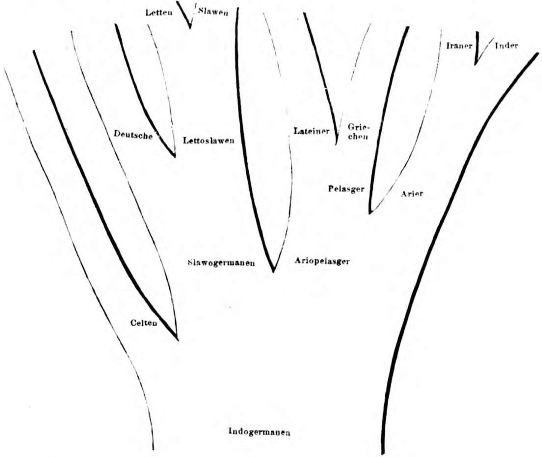
</p>

<p><img src="/images/stammbaum.png" alt="" /></p>

<p><strong>Figure 1</strong>. August Schleicher’s “stammbaum” diagram of languages, published in 1853 (predating Darwin’s <em>On the origin of Species</em> by 6 years).</p>

<p>So anyway, back to these computational phylogenetic methods. You need data, you need an evolutionary model (a mathematical framework describing how the data evolves), and you need a computer that can crunch the numbers and give you a tree (or perhaps a whole forest of trees). For data, biologists have been able to benefit from huge strides in genetics and genomic sequencing in recent decades. Genetic data has largely replaced <a href="https://en.wikipedia.org/wiki/Morphology_(biology)">morphological data</a> for inferring phylogenetic trees of species. In linguistics, the question of what to use for data is a little more open-ended. By far the most common strategy is to use <em>lexical cognate data</em>. This involves binarising the kinds of congnate sets we encountered in the previous section. A language gets a ‘1’ if it includes a word in a particular cognate set or a ‘0’ if it does not. For example, if we jump back to the table of words for ‘father’ above, each of those languages, Sanskrit, Latin, Ancient Greek, Italian, English and German, would all be coded with a ‘1’ which signifies that they all contain a cognate word related to that proto-Indo-European word <em>*pH₂tér-</em>. Other languages that use unrelated words for father, for example Nepalese (बुबा, <em>Bubā</em> = father), would be coded with a ‘0’. Go through and code all cognate sets for 100–200 basic meaning categories and you get a very large table of 1s and 0s for each language of study.</p>

<p>Bayesian computational methods are the state of the art for turning these spreadsheets of binary cognate data into phylogenetic trees. This allows you to specify prior knowledge in the evolutionary model. For example, you might have archaeological evidence tying a language to a particular time and place. You can include this information to constrain the kinds of trees the software will produce accordingly. There are a whole bunch of details in the evolutionary model that can be played with, governing things like evolutionary rates (how frequently 1s and 0s can change through time), whether and how these rates can vary in different parts of the tree, the relative likelihood of a 0 turning to a 1 versus a 1 turning to a 0 and so forth. Once the model is set up nicely, it’s time to hit the big red button and let the computer run a <em>Markov Chain Monte Carlo</em> process (MCMC). The reason for this is that there are practically infinite ways that a set of languages bigger than a small handful can be linked in a phylogenetic tree. It would be impossible to test every single possible tree. The MCMC process is a genius method for searching just a small subset of all the possibilities in a principled way, honing in on a high-likelihood solution.</p>

<p>MCMC works like so. The computer produces a family tree linking all the languages at random — besides adhering to any tree constraints you might have specified previously, it’ll literally just produce a big random set of bifurcating branches linking everything up. Then it calculates how likely this tree would be given the evolutionary model and the language data. As you can imagine, this random tree is almost certainly nonsense and thus the likelihood score will be low. Next, it produces another random tree and calculates a new likelihood score for the new tree. If the likelihood score is better (or even just very slightly below*) the previous likelihood score, the new tree ‘wins’ that round and the previous tree is discarded. If not, the new tree is discarded and the previous tree is retained. Then the computer produces another random tree and repeats the process. And then it repeats it again. And again. Millions and millions of times. In a pinch, you might be able to get away with 10 million iterations, but for anything publication quality you’re really looking at 100 million or more. Obviously, the first many iterations are junk, but the truly remarkable thing is how quickly and efficiently this MCMC process searches the probability space, narrows in and stabilises around the best solution.
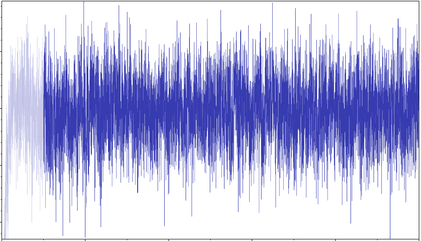
</p>

<p><img src="/images/mcmc_trace.png" alt="" /></p>

<p><strong>Figure 2</strong>. A relatively well behaved MCMC chain. This kind of trace diagram shows the likelihood score for each iteration from the first iteration on the left to the 100 millionth iteration on the right. You can see it starts off pretty wild in the burn-in period, which is why we discard the first 10% (greyed out on the left) but quickly stabilises.</p>

<p>At the end, you’re left not with one single best tree but a whole forest of millions of trees, one from each MCMC iteration. Typically, you discard the first 10% or so as ‘burn-in’ (when the computer is just starting out exploring the probability space and starts off with junky trees before finding better solutions), then you take every 1000th tree (or 2000th or 10,000th tree or so, whatever works) so you end up with a final sample of at least a thousand, perhaps several thousand, high quality, high likelihood trees to work with.</p>

<p>Why not simply take the very last tree, the final ‘winner’ with the highest likelihood of all? Well, the issue is that although, yes, the final tree will have a good likelihood score, the second last tree will also have a very high likelihood score, only very slightly less than the final tree. And so who’s to say that the second last, or the third last tree (and so on) aren’t actually more accurate than the final one? By working with a whole sample, or forest, of trees, which are all quite similar and all quite high likelihood, we get an indication of <em>phylogenetic uncertainty</em>. We’re accepting the fact that we don’t know the one true, historical tree — these are just our best estimates, and the best representation of the real, true tree probably lies somewhere in that forest but we can’t be sure exactly where. If we want a nice family tree figure for the family of languages, there are ways of averaging this forest into a kind of single best average tree like <a href="https://www.nature.com/articles/s41559-018-0489-3/figures/2">this one</a>, complete with confidence levels indicated on each node, which is really nice.</p>

<p>*Why ever accept a tree with a <em>slighly lower</em> probability than the tree before? Just to add a degree of flexibility. Otherwise the MCMC process tends to get stuck on a particular peak in the probability space and start going around in circles. You’ve got to allow it to accept slighly lower probability trees occasionally so it can go down again and properly explore the probability space around it. Otherwise if it gets stuck on the first peak, it might never find the even bigger peak that lies just over a valley below.</p>

<h1 id="the-limits-of-cognate-data">The limits of cognate data</h1>

<p>Over the last 20 years or so, linguists have had a tremendous degree of success inferring language phylogenies using cognate data using the methods described above. You can now find phylogenies for major language families in most parts of the world, including the Indo-European (multiple times), Pama-Nyungan, Austronesian, Bantu, Sino-Tibetan families, and more.</p>

<p>Nevertheless, there are some limitations. Perhaps the biggest one is just how difficult and time consuming cognate data is to acquire. Coding enormous tables of thousands of cognates is hard work. It’s also a job that requires a good deal of familiarity with the languages at hand, in order to discern which words are likely related to others (and, for example, which words look somewhat similar but are more likely to be chance resemblances or borrowings).</p>

<p>One of the results is that, although language phylogenies have been inferred for a good assortment of major language families around the world, there are buckets more language families for which this work remains undone. For example, we have some nice phylogenies of the Pama-Nyungan family, the biggest language family in Australia, but not for the plethora of smaller families packed into the Top End and Kimberley regions. New Guinea, arguably the most linguistically diverse place on earth, remains practically untouched by phylogenetic methods.</p>

<h1 id="phonotactics">Phonotactics</h1>

<p>All human languages have rules about how sounds are allowed to fit into syllables and words. Languages will forbid certain sounds from ever appearing together in sequence. This system of rules is called <em>phonotactics</em>. Phonotactics is language specific; some languages are highly restrictive about what they allow and others are perfectly happy with long, complex consonant clusters. For example, consider the sequence ‘sf’. English never allows words to start with ‘sf’, it just doesn’t work. Italian is perfectly happy to let words start with ‘sf’ though (e.g. <em>sforzo</em>, effort). Likewise, Italian words can start with ‘sb’ (e.g. <em>sbaglio</em>, mistake) which isn’t allowed in English.</p>

<p>One of the things that makes phonotactics interesting from a historical perspective is that phonotactic restrictions tend to be quite resilient. A language’s <em>lexicon</em>, from which we get cognate data, is changing all the time as speakers of the language invent new words, borrow words from neighbouring languages, and send old words out of fashion. Borrowings can be particularly problematic for phylogenetic methods, because they can get erroneously marked as cognates (as if two languages both inherited the word from a common ancestor rather than one language borrowing the word from the other).</p>

<p>Phonotactics, by contrast, is a bit more historically conservative. That’s not to say phonotactic rules <em>never</em> change — they can and do change sometimes. But we can observe languages preserving phonotactic restrictions even as they borrow vocabulary from other languages. Some of my favourite examples illustrating this come from the word ‘Christmas’ rendered into different languages. Japanese, which is incredibly restrictive about consonant clusters and never allows words to end with a vowel, turns ‘Christmas’ into <em>kurisumasu</em>, with a heap of vowels inserted to break those consonant clusters up. As Bing Crosby teaches us, ‘Merry Christmas’ in Hawaiian is <em>meli kalikimaka</em>, which is the result of applying both Hawaiian’s strict (C)V(V) syllable structure (C = consonant, V = vowel, brackets = optional) and famously constrained phoneme inventory (in which English’s ‘l’ and ‘r’ sounds both belong to the same sound category, and there is no ‘s’ sound). So we see that even though these languages both borrowed the word ‘Christmas’, they adapted it to fit existing phonotactic restrictions.</p>

<p>One of the other interesting things about phonotactics is that you can extract a lot about a language’s phonotactics straight from a wordlist, and you can even automate large parts of the process. You can tell a lot about which sequences of sounds are allowed to go together and which sequences never go together just by seeing which sequences appear in the language’s wordlist and which don’t. This means you can get a large volume of data fairly quickly using computers, without the need to make complex cognate judgements, and you can do so even for languages that are understudied and under-resourced, just as long as you’ve got a decent list of words.</p>

<h1 id="my-research-question">My research question</h1>

<p>So, at last, we get to the overarching research question driving my PhD. I wanted to know whether I could combine existing <em>cognate</em> data with new <em>phonotactic</em> data to infer phylogenetic trees of languages, using the Pama-Nyungan family as a test case. Testing this is simple enough in essence: Infer a tree using cognates, infer a tree using cognates and phonotactic data, and see which one “wins”. Of course, testing this question was quite a bit more complex in practice, but that’s the idea.</p>

<p>To be clear, the goal is not to create a silver bullet method for automatically inferring trees just from simple wordlists. Cognate data is, and will remain, tremendously valuable. If inferring trees with phonotactics worked, it would mean we’d have an extra nifty source of data to <em>complement</em> cognates and other lines of evidence.</p>

<p>Because this post has already become quite lengthy, I’ll leave it here on a cliffhanger. In a Part II follow-up, I’ll discuss the papers I wrote as part of my thesis, what I found, the difficulties I faced and what it all means. Thanks for sticking around!</p>]]></content><author><name>Jayden Macklin-Cordes</name><email>jayden@macklin-cordes.com</email></author><category term="PhD life" /><category term="linguistic phylogenetics" /><category term="Australian languages" /><summary type="html"><![CDATA[My PhD thesis, with the catchy title Phonotactics in historical linguistics: Quantitative interrogation of a novel data source, is now available (open access) on UQ eSpace.]]></summary></entry></feed>