A few years ago, I did the thing where you write the thing, and now I’m legally entitled to sow confusion by shouting “I’m a doctor!” during medical emergencies on planes¹. In a previous post (Part I), I wrote about the background and motivation behind the PhD project that kept me busy for so long. But I left it on a cliffhanger. The big question driving my PhD was whether I could build better family trees of languages (phylogenies) by combining traditional cognate data (sets of related words across languages) with a new kind of data extracted from phonotactics, the rules governing which sounds are allowed to appear together. At the end of the post, I promised a Part II discussing what I actually found. Four short years later, here it is. I appreciate your patience.

To briefly recap: the appeal of phonotactic data is twofold. First, a language’s phonotactic restrictions tend to be historically conservative — even when languages borrow vocabulary from their neighbours, they tend to reshape those borrowed words to fit their own sound rules (I’m sure you all remember the kurisumasu and meli kalikimaka examples from Part I like it was yesterday 😉). Second, you can extract a lot of phonotactic information straight from a wordlist using automated methods, which is a huge advantage for understudied language families where detailed cognate data doesn’t yet exist.

Before I could answer the main question, though, I had to do some groundwork. I needed to understand the data itself — what does it look like, statistically? Then I needed to check whether phonotactic data actually carries any historical information at all, before attempting to feed it into a tree-building algorithm. Only then could I run the big experiment. What follows is the story of that process. And, fair warning, the ending isn’t quite the fairytale I expected.

What does the data actually look like?

Before you pour data into a fancy algorithm, you should probably understand the data itself. What shape does it have? What patterns does it follow? What does that tell you about the forces that produced it? This is the eat-your-vegetables portion of the thesis — not the flashiest part, but it earns its place later.

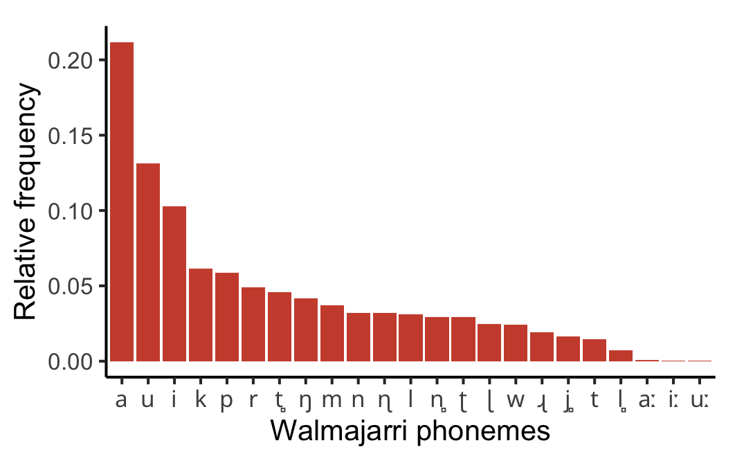
Here’s the question. Every language has a set of contrastive speech sounds — its phonemes. Some of those phonemes are very common in the language’s vocabulary and others are quite rare. If you rank a language’s phonemes from the most frequent to the least, what pattern do you get? Is it a gentle slope, with most sounds appearing at roughly similar rates? Or is it something more dramatic?

It turns out to be dramatic. The pattern you see, again and again across different languages, is a sharply skewed curve: a handful of phonemes are extremely common, and then there’s a long tail of many phonemes that are relatively rare. If you rank UK cities by population, you get a similar kind of shape (Figure 1). London towers over everything, Birmingham and Manchester are a distant second and third, and then there’s a long, flat tail of dozens of cities from Leicester down to Guildford that are all roughly the same size relative to London. This kind of heavily skewed distribution pops up all over the place in nature and human society, from the popularity of websites to the distribution of earthquake magnitudes. In linguistics, it’s associated with George Zipf, who observed that word frequencies in a text follow a similar pattern (the most common word appears roughly twice as often as the second most common, three times as often as the third, and so on) — hence you may hear references to “Zipfian” distributions, or “Zipf’s Law”.

Previous researchers had claimed that phoneme frequencies follow this same Zipfian pattern. But there was a problem: the statistical methods they’d used to evaluate this had since been shown to be unreliable. So, using more robust methods and a dataset of 166 Australian languages, I re-evaluated the question. What I found was more nuanced than the earlier picture. The most frequent phonemes in a language do follow something like a Zipfian, power law pattern — a “rich-get-richer” dynamic where the already-common sounds tend to attract even more usage. But the least frequent phonemes follow a different pattern entirely, one better described by an exponential distribution, which is associated with simpler “birth-death” processes where sounds come and go at some characteristic rate. In other words, a kind of split personality: one pattern governing the top of the frequency ranking and a different pattern governing the bottom.

Why should we care about any of this? Two reasons. First, different mathematical distributions point to different underlying causal processes. If we can identify the right distribution, we’re getting a clue about the forces — sound changes, borrowings, mergers, splits — that shape a language’s phoneme inventory over time. That’s intrinsically interesting, but it also matters practically, because if you want to build an evolutionary model of how these frequencies change along a family tree, you need to know what you’re modelling. Second, this result was an early warning sign. The data has a complex, composite structure — it doesn’t follow one neat pattern — and that means capturing it faithfully in a statistical model is going to be difficult. A point I would come to appreciate more fully later on.

Is there a trace of history in phonotactics?

The previous section looked at the frequencies of individual sounds. A useful starting point, but not quite where the action is. Remember, it’s phonotactics that I hypothesised to be historically conservative — the rules governing which sounds are allowed to appear together, not just how often individual sounds crop up. So the natural next step was to turn to the frequencies of sequences of sounds, pairs of adjacent segments called biphones. This also has the happy side effect of giving far more data to work with per language (a language might have only 20-odd phonemes, but hundreds of biphone sequences). It’s all very well that phoneme frequencies have interesting statistical properties. But the real question for my project is whether phonotactic data, the rules and frequencies governing how those phonemes fit together, actually contain historical information. Do closely related languages resemble each other phonotactically more than distant ones? If not, the data is just noise as far as phylogenetics is concerned, and I can pack up and go home.

The concept I needed is called phylogenetic signal. The idea is simple enough: if some trait has evolved along a family tree, then closely related species (or languages) should resemble each other more than distantly related ones, and more than you’d expect by chance. Think of it like family resemblances. Siblings tend to look more alike than cousins, who tend to look more alike than strangers². That’s a consequence of shared ancestry — more specifically, the relative amount of shared ancestry (siblings have shared ancestry down to the parent generation, cousins have shared ancestry down to the grandparent generation). The same logic applies to languages. If phonotactics evolves along a language family tree, then closely related languages should have more similar phonotactic patterns than distant relatives. And crucially, there are statistical tests that let you quantify this — to measure not just whether the resemblance is there but how strong it is.

So I took phonotactic data from 112 languages from the Pama-Nyungan family, a large family of Indigenous Australian languages spanning about 90% of the continent. I then compared the data against a known family tree that had been built independently from cognate data (the traditional, gold-standard way to build language trees). The test: does the phonotactic variation across these languages line up with what we’d expect if it had evolved along that tree? I ran this test on three progressively finer-grained datasets. The first was binary — for each pair of adjacent sounds (a biphone), does it occur in a language’s vocabulary or not? This is the coarsest level of information: a simple yes or no. The second recorded the actual frequencies of transitions between individual sounds — not just whether a sequence occurs, but how often. The third grouped sounds into natural classes (categories like “nasal” or “velar” that reflect how and where in the mouth a sound is produced) and recorded transition frequencies between those classes.

The result was clear, and if it wasn’t yet time to pop some champagne corks, it was at least time to grab a couple of bottles and put them on ice. All three datasets showed statistically significant phylogenetic signal. But the strength of that signal increased markedly as the data got more fine-grained. The binary data — the simple yes-or-no — showed the weakest signal. The frequency data was stronger. And the natural-class-based frequency data was strongest of all. This makes intuitive sense: there’s far more information in how often a sound sequence occurs than in merely whether it occurs. And grouping sounds into natural classes captures something real about how sound change actually works — sound changes tend to affect whole classes of sounds (all the nasals, say), not just individual phonemes one at a time.

What made this result especially striking is that Australian languages have long been described as phonotactically uniform. The conventional wisdom was that there just wasn’t much phonotactic variation to find. And at a coarse, binary level, that’s partly true — many of the same sound sequences are permitted across most Australian languages. But once you look at the frequencies, a different picture emerges. There’s a rich layer of variation hiding beneath the surface, and that variation patterns phylogenetically. The historical signal was there all along; you just needed the right resolution to see it.

So, phonotactics carries genuine historical information. In principle, this data could help build better family trees of languages. I could stop here, on this high note, and give the impression that phonotactics is the answer to all our phylogenetic prayers. But that would be only half the story. Don’t pop those champagne corks just yet…

The big experiment

Time for the real test. But detecting a signal and using it to infer a tree are very different propositions. To actually put this to the test, I needed to combine phonotactic data with traditional cognate data, feed both into the Bayesian tree-building machinery, and see whether the result was any better than what you’d get from cognates alone.

Back in Part I, I gave some background on Bayesian computational approaches to phylogenetic tree inference. And, in particular, I described a process called MCMC (Markov Chain Monte Carlo), where the computer generates millions upon millions of random trees and gradually homes in on the best solutions. This is the approach I took here. It’s finally time to see it in action. I set up two competing models for a sample of 44 western Pama-Nyungan languages. In the first model, the computer builds a single tree from both the cognate data and the phonotactic data together. In the second, it builds two separate trees — one from cognates, one from phonotactics — independently of each other. If the phonotactic data genuinely helps, then the combined model should fit the data better than keeping the two data sources apart. The method for comparing models is technical, but the underlying question is simple: does adding phonotactic data make the tree better, or not?

It did not.

Or, more precisely: the experiment failed to produce a clear answer, which is arguably worse than a clean negative result. The models with phonotactic frequency data never properly stabilised. Remember those MCMC trace plots from Part I — the ones that show the computer’s likelihood score at each iteration, and how they’re supposed to settle into a nice, stable plateau? Mine looked like abstract art. Some chains would wander around aimlessly for tens of millions of iterations. Others would appear to converge, then abruptly lurch somewhere else. No amount of praying to the Bayesian gods would suffice to make them behave. The upshot is that the statistical comparison between models was unreliable. I couldn’t trust the numbers.

What I could glean from the wreckage was not encouraging. The best average tree produced by the combined model came out oddly flat — a squished, star-like structure with weaker branching than you’d get from cognates alone. In tree-building, a flat tree is a tree that’s not really saying much. It’s the phylogenetic equivalent of a shrug. This suggested that the phonotactic data, rather than adding useful historical signal, was introducing a bunch of noise that washed out the branching structure.

Why did it go wrong? The core problem was a tension between making the evolutionary model realistic and making it computationally feasible. The model I used assumed that phonotactic frequencies change gradually over time — drifting up and down at random, a process called Brownian motion. This is a reasonable starting point and it’s a standard model available in existing phylogenetic software. But real sound change doesn’t work like that. When a language undergoes, say, a phonemic merger (two formerly distinct sounds collapse into one³), the frequencies of affected sound sequences don’t drift gently downward. They jump, suddenly, to zero or one. And when new sound distinctions emerge, the reverse happens: frequencies leap from zero to some non-trivial value overnight. A model that only allows for gradual drift is going to struggle with data that’s shaped by sudden jumps. On top of this, I had to treat every phonotactic variable as if it were evolving independently of every other — which is linguistically absurd, since sound changes affect whole classes of sounds at once. But modelling the dependencies between thousands of variables would have been computationally intractable. So I made the simplification, knowing it was wrong, because the alternative was not running the experiment at all.

This is not the fairytale ending you want for the final chapter of your PhD. Put that champagne back in the fridge.

What I learned

A PhD that ends with “it didn’t work” sounds dispiriting (and trust me, I’ve spent plenty of time feeling dispirited about it). But, especially with some time and distance to reflect, I realise that isn’t quite right. The result was indeterminate, not negative. The experiment didn’t show that phonotactics is useless for phylogenetics — it showed that the tools I had weren’t yet adequate for the job. Those are very different conclusions, even if they felt similar at 2am during the depths of late-stage thesis-writing hell.

“If you’ve made up your mind to test a theory, you should always decide to publish it whichever way it comes out. If we only publish results of a certain kind, we can make the argument look good. We must publish both kinds of results.” — Richard Feynman

I take this seriously. If I’d stopped after the phylogenetic signal paper — the beautiful positive result — and never attempted the tree inference experiment, I’d have left a misleading impression that phonotactics was ready for phylogenetic prime time. It isn’t. Not yet. And the field is better served by knowing that than by not knowing it. So did I really spend nearly 5 years of my life investigating a kinda out-there question, which no one was asking, only to find, uh, nothing? I don’t think it’s quite that bleak!

The thesis offers three main contributions. First, it demonstrated that phonotactic data carries genuine historical signal — that the patterns in which sounds are allowed to fit together reflect the evolutionary history of a language family, even in a part of the world where phonotactics was assumed to be boringly uniform. That result stands. Second, it showed that fine-grained frequency data is far richer than coarse binary data for this purpose. If you just ask “does this sound sequence occur: yes or no?” you get a faint signal. If you ask “how often?” you get a much stronger one. Third — and this is the contribution I’m most invested in — it laid out a principled, step-by-step methodology for evaluating any new kind of data in phylogenetics. Rather than just slurping up whatever data we can get our hands on and pouring it into a computational black box, the thesis argues for a deliberate progression: understand the data’s statistical structure, test for phylogenetic signal, evaluate the evolutionary dynamics, and only then attempt tree inference. That framework is generalisable beyond phonotactics.

As for the tree inference question itself, it remains open. To revisit it properly, future work would need better evolutionary models — ones that account for the sudden jumps of sound change rather than assuming everything drifts gradually. It would need smarter ways of handling the dependencies between phonotactic variables, perhaps through phylogenetic factor analysis or linguistically motivated data partitioning. And it would benefit from advances in computational power that are already underway. The problem is hard, but it doesn’t look intractable.

Phylogenetic methods in linguistics are still maturing, and that means you often find yourself innovating, customising or building tools from scratch on the way to answering the question. This can be challenging, but it’s also where the most rewarding work tends to happen. There’s a wide gap between “this data contains useful information” and “we can successfully use this data in a model,” and bridging it requires the kind of slow, methodical groundwork that doesn’t make for a flashy conference talk — but without which the flashy results would be built on sand. For the sake of the world’s under-resourced languages, and the histories they encode, that bridging work is worth doing. And it’s far from finished.